Lower Layers (5): Erasure-Coding Math, from GF(2⁸) to FastEC
TL;DR this chapter in a few lines
- Erasure coding in Ceph is arithmetic in GF(2⁸): each byte is a field element, addition is XOR, and multiplication uses log tables.
- Encoding multiplies the data chunks by a generator matrix; Reed–Solomon matrices keep any k shards enough to decode (the MDS property).
- Decoding after a loss inverts the matching rows of the matrix; parity-delta updates change parity without reading the whole stripe.
- Tentacle's FastEC uses this for partial reads and writes, behind
allow_ec_optimizations.
27-1 Introduction: from XOR to Reed-Solomon#
In chapter 13 we saw how a pool with erasure coding is created and what the profiles mean. This chapter goes one layer lower: the mathematics of the finite field , building the Reed-Solomon generator matrix (with the Vandermonde and Cauchy methods), the SIMD implementation in ISA-L, and how Ceph splits an object into stripes and chunks, performs partial writes with read-modify-write, and what changed in Tentacle with optimized EC (usually called FastEC). We also work through a complete numerical example of encode and decode by hand.
- All the main plugins (isa, jerasure and the base of clay) work in . In this field addition is XOR and multiplication is done with log/exp tables or SIMD.
- The default profile in Tentacle and main is
plugin=isa technique=reed_sol_van k=2 m=2. In Squid the default wasplugin=jerasure. - In ISA-L, Vandermonde is guaranteed MDS only for m ≤ 4 (and for m=4 only with k ≤ 21). Otherwise Ceph switches to
cauchyautomatically. - The default
stripe_unitis 4K, and it becomes 16K for pools withallow_ec_optimizations. - Optimized EC in Tentacle (
ECSwitchbetween the old and the new backend) makes direct partial reads and parity updates with a delta possible. Once enabled, it cannot be disabled.
27-2 GF(2⁸): arithmetic on bytes#
Erasure coding has to "multiply and divide" bytes in such a way that every non-zero number has an inverse and the result always stays a byte. The Galois field provides exactly that. Its elements are the 256 bytes, viewed as polynomials of degree less than 8 with coefficients 0 and 1.
- Addition and subtraction: both are XOR, so a + a = 0.
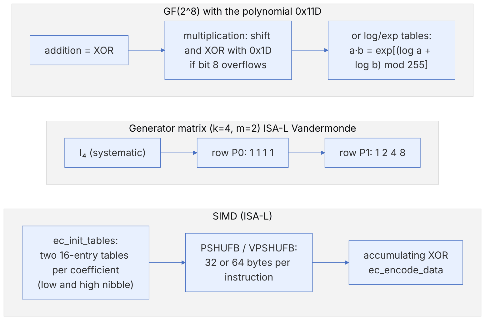
- Multiplication: the polynomials are multiplied and then reduced modulo an irreducible polynomial of degree 8. ISA-L uses 0x11D (x⁸ + x⁴ + x³ + x² + 1): on each left shift, if bit 8 becomes set, the value is XORed with 0x1D (the same pattern for multiplying by 2 can be seen in
ec_base.c). - log/exp tables: because 2 is a generator of the multiplicative group, every non-zero byte equals . So and .
| Sample multiplication in with 0x11D | Result | Explanation |
|---|---|---|
| 0x02 × 0x04 | 0x08 | no overflow; just a shift |
| 0x34 × 0x02 | 0x68 | 0x34 << 1 = 0x68 |
| 0x56 × 0x04 | 0x45 | 0x56 << 2 = 0x158 → bit 8 set → 0x58 ⊕ 0x1D = 0x45 |
| 0x78 × 0x08 | 0xE7 | three shifts with two overflows |
27-3 Systematic Reed-Solomon#
In a systematic (k, m) code, the k data chunks are stored unchanged and m parity chunks are computed from them. If D is the data vector, the chunks are obtained by multiplying the (k+m)×k generator matrix G by D: C = G · D. The first four rows of G are the identity. The code is MDS, meaning any k of the k+m chunks are enough for reconstruction, provided every k×k submatrix of G is invertible.
ISA-L's gf_gen_rs_matrix builds parity row i from the powers of . This is a simple "Vandermonde" matrix that is not MDS for every (k, m). That is why ErasureCodeIsa.cc, if m > 4 or m = 4 and k > 21, logs a message and switches to gf_gen_cauchy1_matrix, whose entries are 1/(i ⊕ j) and which is always MDS. The upper limit for k is MAX_K = 32.
| Parity matrix for k=4, m=2 | Row P0 | Row P1 |
|---|---|---|
| ISA-L reed_sol_van | 1 1 1 1 | 1 2 4 8 |
| ISA-L cauchy | 0x47 0xA7 0x7A 0xBA | 0xA7 0x47 0xBA 0x7A |
27-3-1 Complete example: encoding a small stripe#
Suppose each chunk has only one byte and the data is D = (0x12, 0x34, 0x56, 0x78) (in reality the same computation is repeated for every byte of the 4K chunks):
P0 = 1·12 ⊕ 1·34 ⊕ 1·56 ⊕ 1·78 = 12 ⊕ 34 ⊕ 56 ⊕ 78           = 0x08
P1 = 1·12 ⊕ 2·34 ⊕ 4·56 ⊕ 8·78 = 12 ⊕ 68 ⊕ 45 ⊕ E7           = 0xD8
chunks = [12, 34, 56, 78 | 08, D8]   (shard 0..5)
27-3-2 decode: losing two shards#
Suppose the OSDs holding D1 and D3 have been lost and the healthy shards are {D0, D2, P0, P1}. The corresponding rows of G form a 4×4 matrix. Its inverse is computed in (ISA-L uses gf_invert_matrix), and the rows for the missing data are multiplied by the healthy bytes:
D1 = 7B·D0 ⊕ F5·D2 ⊕ A6·P0 ⊕ DD·P1 = 0x34   ✓
D3 = 7A·D0 ⊕ F4·D2 ⊕ A7·P0 ⊕ DD·P1 = 0x78   ✓
All the numbers in these two sections were computed and checked with an independent Python implementation of with 0x11D and the same matrix-building algorithm as ISA-L. The decode coefficients are computed only once for each failure pattern, and the isa plugin keeps them in ErasureCodeIsaTableCache, because inverting the matrix is more expensive than encoding.
Why is SIMD so fast? Multiplying a byte x by a constant c can be split into two nibbles: c·x = c·(x_hi << 4) ⊕ c·x_lo. Each has only 16 possible values, so two 16-byte tables are enough. The PSHUFB instruction (or VPSHUFB in AVX2/AVX-512) can perform 16, 32 or 64 simultaneous lookups in a 16-byte table. ISA-L builds these tables for all the coefficients with ec_init_tables, and ec_encode_data runs the multiply and the accumulating XOR with these instructions for each input block. The result is an encode speed of several gigabytes per second per core. jerasure (with gf-complete) uses a similar method, but ISA-L is usually faster on x86. The isa plugin also works on Arm, with ISA-L's NEON and SVE code.
27-4 Stripes, chunks and layout on the OSDs#
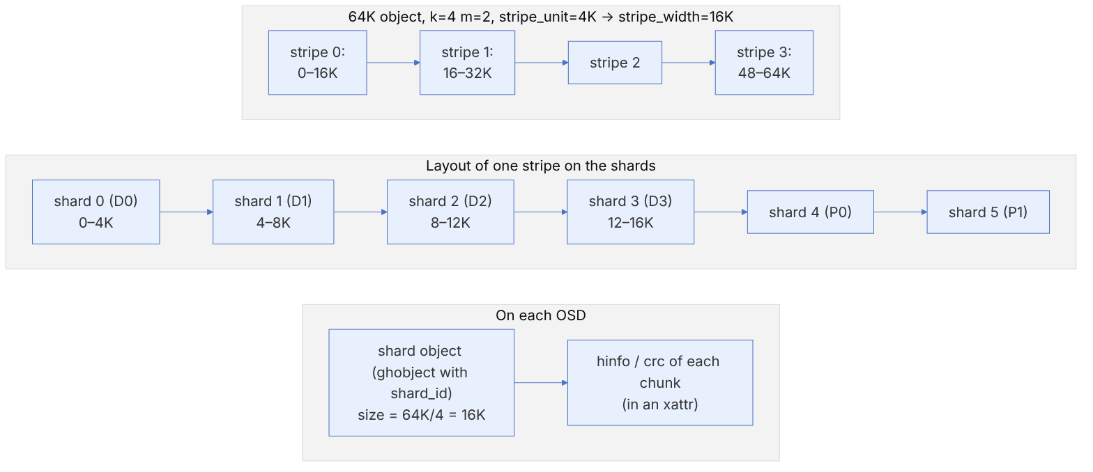
| Concept | Definition | Default |
|---|---|---|
stripe_unit (chunk size) | the data bytes of one shard in one stripe | 0 in osd_pool_erasure_code_stripe_unit, meaning 4K, or 16K if the pool is optimized and the plugin supports it |
stripe_width | k × stripe_unit | for k=4: 16K or 64K |
| shard object | ghobject_t with shard_id of 0..k+m−1 | on the OSD with an onode key containing shard + 0x80 (chapter 24) |
ceph osd pool create rejects the profile without --yes-i-really-mean-it if stripe_unit is not a multiple of 4K. Choosing a larger stripe_unit means more writes smaller than one stripe, but more efficient sequential reads. With optimized EC this trade-off has moved towards 16K, because a partial write no longer reads the whole stripe.
27-5 read-modify-write in the old EC#
Up to Squid, and in pools without optimizations in later releases, the EC backend does the following for every write that does not cover a whole stripe and lands on existing data (allow_ec_overwrites=true, required for RBD and CephFS):
pseudocode: partial overwrite in the old ECBackend (this book's summary)
  extent = round_out(write, stripe_width)              # widen to the stripe boundary
  if cache miss: read k chunks of extent from shards   # several network round trips
  merge new bytes into stripe buffer
  encode → m parity chunks for whole stripe
  send sub-writes to all k+m shards (each shard, its own transaction)
  wait all commits → reply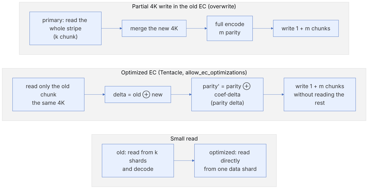
Why is the parity delta correct? Because the code is linear: . If only changes to , then . With the example from the previous section, if D1 changes from 0x34 to 0x35, the delta is 0x01, so P0′ = 0x08 ⊕ 1·0x01 = 0x09 and P1′ = 0xD8 ⊕ 2·0x01 = 0xDA. There is no need to read D0, D2 and D3.
Plugin flag (ErasureCodeInterface.h) | Meaning |
|---|---|
FLAG_EC_PLUGIN_PARTIAL_READ_OPTIMIZATION | the code is systematic; a small read goes directly to the data shard |
FLAG_EC_PLUGIN_PARTIAL_WRITE_OPTIMIZATION | a write smaller than one chunk needs only that piece from each data shard |
FLAG_EC_PLUGIN_ZERO_INPUT_ZERO_OUTPUT_OPTIMIZATION | all-zero data gives zero parity (for empty regions) |
FLAG_EC_PLUGIN_ZERO_PADDING_OPTIMIZATION | zero-length buffers are allowed |
FLAG_EC_PLUGIN_PARITY_DELTA_OPTIMIZATION | parity update with a delta |
FLAG_EC_PLUGIN_REQUIRE_SUB_CHUNKS | the plugin needs sub-chunks (CLAY) |
FLAG_EC_PLUGIN_OPTIMIZED_SUPPORTED | can be used in an optimized pool: isa, and jerasure only with reed_sol_van |
# Tentacle and later:
ceph osd erasure-code-profile set ec42 plugin=isa technique=reed_sol_van k=4 m=2 crush-failure-domain=host
ceph osd pool create ecdata erasure ec42
ceph osd pool set ecdata allow_ec_overwrites true
ceph osd pool set ecdata allow_ec_optimizations true     # irreversible
ceph osd pool get ecdata all | grep -E 'ec_optim|stripe'FLAG_EC_OPTIMIZATIONS is defined in osd_types.h with the comment "once enabled, cannot be disabled". Before enabling it on a production pool, make sure all OSDs have been upgraded to a release that supports it. Try it first on a test pool. osd_pool_default_flag_ec_optimizations (default false) controls whether it is enabled automatically for new pools.
27-6 Codes with lower repair bandwidth#
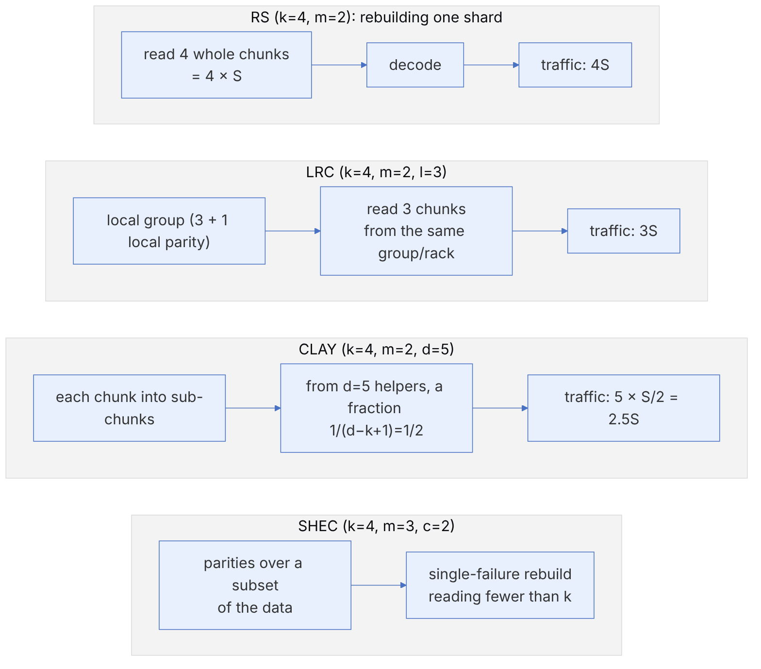
In RS, rebuilding a lost shard requires reading k whole chunks. For k=8 this means 8 times the lost data crosses the network. Three Ceph plugins reduce this cost in different ways:
| Plugin | Parameters (default) | Idea | Trade-off |
|---|---|---|---|
lrc | k, m, l | add a local parity for every l chunks; usually each group in one rack | more space overhead: (k+m)/k + (k+m)/(l·k) |
clay | k=4, m=2, d=k+m−1 (default) | a coupled-layer code with sub-chunks: repair by reading a fraction from d helpers | minimal repair (MSR); the number of sub-chunks is , which grows quickly with k+m, and the reads become tiny |
shec | k=4, m=3, c=2 | each parity covers only part of the data; c = the number of failures guaranteed to be tolerated | space efficiency between RS and replication; cheaper single repairs |
Numerical example for CLAY: the repair bandwidth for one shard of size S is . With k=8, m=4 and d=11 this is 11S/4 = 2.75S, while the equivalent RS reads 8S (about 66% savings). But q = d − k + 1 = 4 and t = (k+m)/q = 3, so each chunk is split into sub-chunks. With a stripe_unit of 4K the sub-chunks are 64 bytes, and the repair read becomes tens of small, scattered reads. That is why CLAY makes sense with a larger stripe_unit.
27-7 crc and integrity in EC#
In the old EC, for append-only pools (without overwrites), a hash of each shard (hinfo_key in an xattr) was kept and deep scrub checked it. With allow_ec_overwrites this hash is no longer updated, and integrity relies on BlueStore's checksums in each shard (chapter 23). Deep scrub in EC reads every shard and checks parity consistency by encoding again. The FLAG_EC_PLUGIN_CRC_ENCODE_DECODE_SUPPORT flag in main indicates that the plugin can compute a crc from the crcs of the data, that is, combine the linearity of crc with the code. This is part of the ongoing work on faster scrub. Check your release before relying on it.
ceph osd erasure-code-profile get default
ceph osd pool ls detail | grep -E 'erasure|stripe_width'
ceph pg <pgid> query | jq '.info.stats.stat_sum.num_objects_degraded'
ceph tell osd.4 config get osd_recovery_max_active_hdd27-8 GF(2⁸) arithmetic at the instruction level: log/exp tables and the nibble trick#
The previous sections defined multiplication in . This section shows how ISA-L, on which Ceph's isa plugin relies, performs this multiplication in the hot loop. ISA-L's reduction polynomial is the same 0x11D (that is, ). In the code this number appears as 0x1d: whenever bit 7 is set before the shift, the result is XORed with 0x1d.
Source in code: isa-l/erasure_code/ec_base.c :: gf_mul, gf_inv
Complexity: O(1): two lookups, one addition and one comparison; tables of 256 + 256 bytes
pseudocode
# built once: exp[i] = 2^i and log[2^i] = i for i in 0..254
x = 1
for i in 0..254: exp[i] = x; log[x] = i; x = x·2 (that is x≪1, and ⊕ 0x11D on overflow)
gf_mul(a, b): if a == 0 or b == 0: return 0
              i = log[a] + log[b]; if i > 254: i −= 255
              return exp[i]
gf_inv(a):   return exp[255 − log[a]]
Numerical example. exp[0..15] = 01 02 04 08 10 20 40 80 1D 3A 74 E8 CD 87 13 26. So , that is, the first overflow. For 0x53 × 0xCA we have log[0x53] = 206 and log[0xCA] = 73. Their sum is 279, and because it is greater than 254, 279 − 255 = 24 and exp[24] = 0x8F. The inverse of 0x02 is exp[255 − 1] = 0x8E. Check: 0x8E × 2 = 0x11C and 0x11C ⊕ 0x11D = 0x01.
This method has two random table accesses and one branch per byte and is slow in the hot loop. That is why ISA-L builds a different table that fits SIMD instructions.
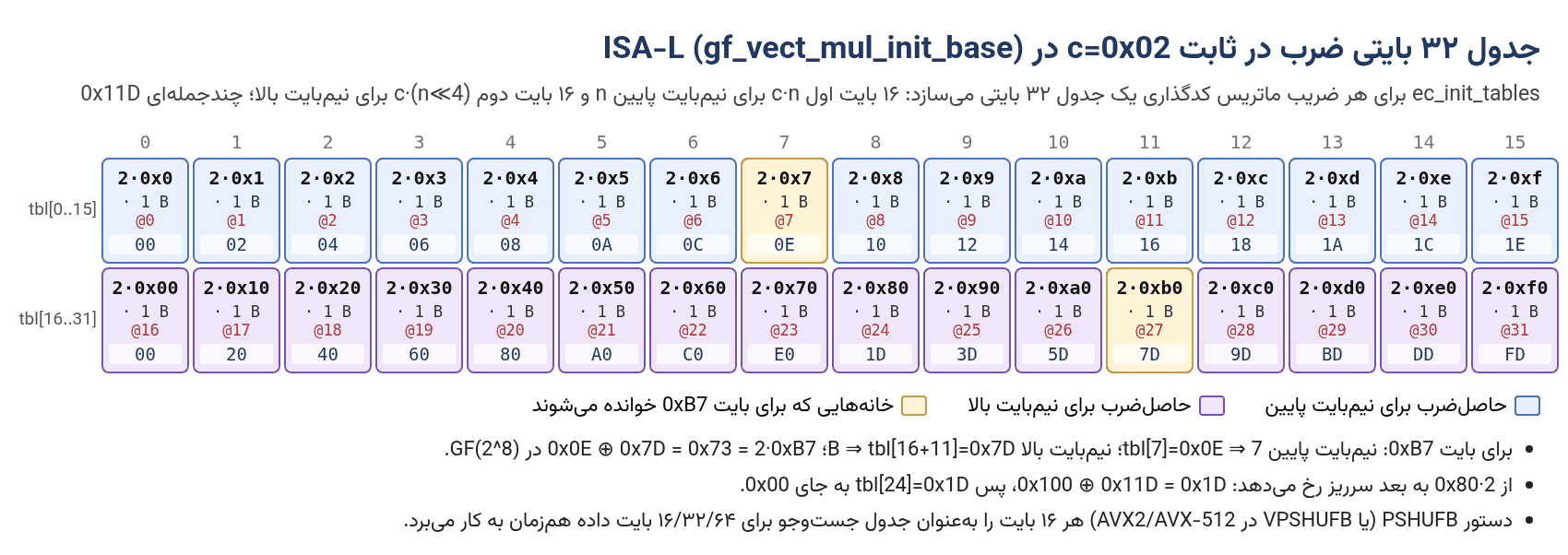
The trick is correct because every byte d equals (d AND 0xF0) ⊕ (d AND 0x0F), and multiplication by c distributes over ⊕. So instead of a 256-entry table for each c, two 16-entry tables are enough. 16 entries is exactly the size of an XMM register, and the PSHUFB instruction works with exactly that size: it takes each byte of the second register as an index into the first.
Source in code: isa-l/erasure_code/ec_base.c :: gf_vect_mul_init_base, ec_init_tables_base and the assembly versions gf_*vect_dot_prod_avx2.asm
Complexity: table construction O(32) per coefficient, that is 32·k·m bytes for the whole matrix. Encoding O(k·m·L/W) instructions for L bytes with register width W (16/32/64)
pseudocode
init(c): for n in 0..15: tbl[n] = c·n ; tbl[16+n] = c·(n≪4)
encode_row(row r, data D0..Dk-1, length L):
    for off in 0, W, 2W, … < L:                 # W = 32 with AVX2
        acc = 0
        for j in 0..k-1:
            v  = load(Dj + off)
            lo = v AND 0x0F ; hi = (v ≫ 4) AND 0x0F
            acc ^= PSHUFB(tbl[r][j].lo, lo) ^ PSHUFB(tbl[r][j].hi, hi)
        store(P_r + off, acc)
Numerical example. For d = 0xB7 and c = 2: the low nibble 7 leads to tbl[7] = 0x0E and the high nibble B to tbl[27] = 0x7D. 0x0E ⊕ 0x7D = 0x73, which matches 2·0xB7 computed directly (0x16E ⊕ 0x11D = 0x73). For k=4, m=2, that is six coefficients, ec_init_tables builds 6 × 32 = 192 bytes of tables. In ErasureCodeIsaDefault::prepare Ceph allocates an array of k·(m+k)·32 bytes and keeps the tables in ErasureCodeIsaTableCache, so that they are built only once for each (k, m). The decode tables are also kept in an LRU of length decoding_tables_lru_length, because each failure pattern needs a different matrix.
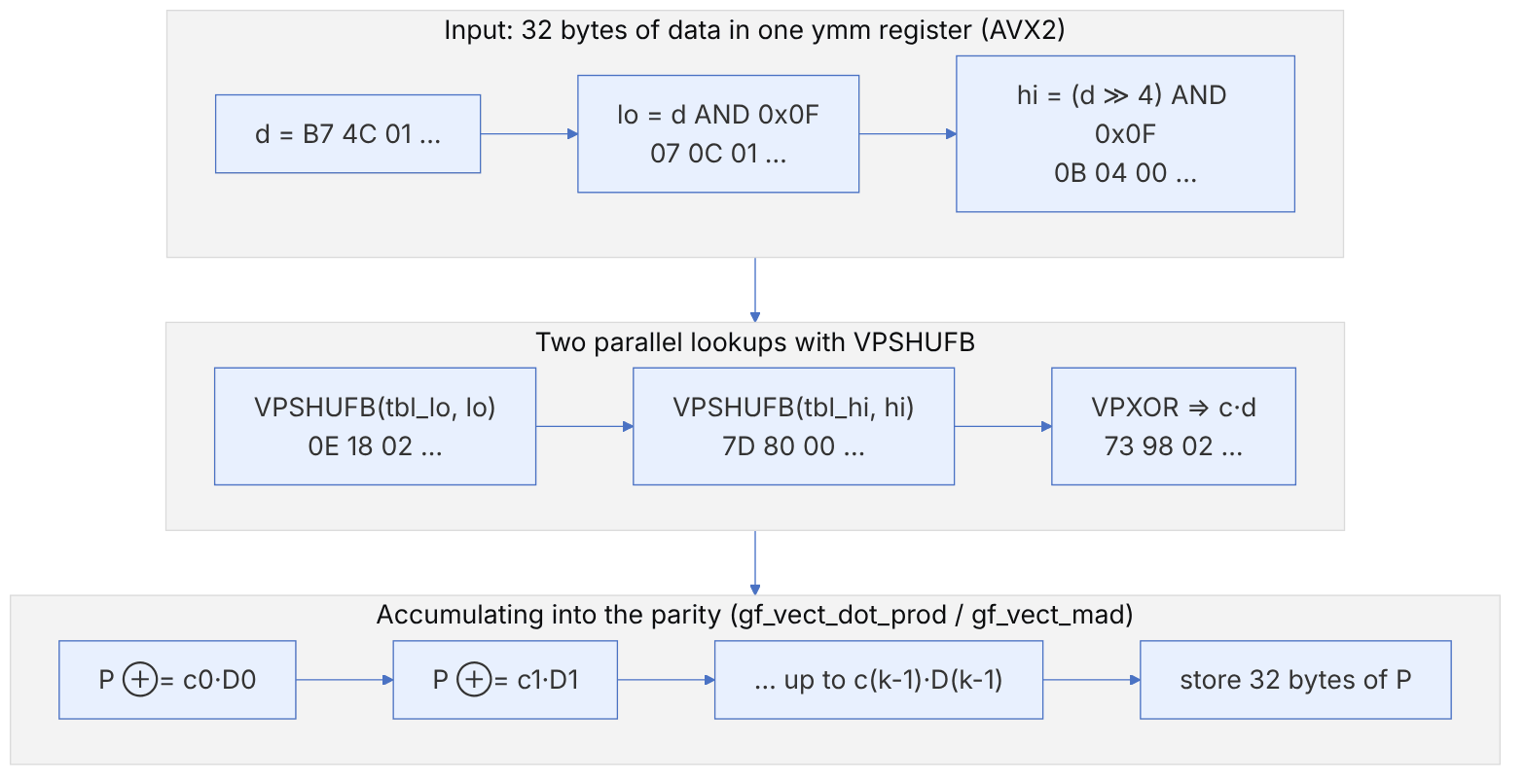
On processors with GFNI, ISA-L chooses the *_gfni.asm versions. The GF2P8AFFINEQB instruction performs multiplication by a constant as an affine transform on each byte and removes the nibble table. The version is chosen at run time by the multi-version dispatcher (ec_multibinary.asm) based on CPUID, not when Ceph is compiled.
27-9 Generator matrices: Vandermonde versus Cauchy#
The isa plugin knows two matrices: technique=reed_sol_van (the default), which calls gf_gen_rs_matrix, and technique=cauchy, which calls gf_gen_cauchy1_matrix. Both build a (k+m)×k matrix with a k×k identity matrix on top, so the code is systematic.
Source in code: isa-l/erasure_code/ec_base.c :: gf_gen_rs_matrix, gf_gen_cauchy1_matrix; src/erasure-code/isa/ErasureCodeIsa.cc :: ErasureCodeIsaDefault::parse, prepare
Complexity: O(k·m) GF multiplications for both
pseudocode
gf_gen_rs_matrix(a, rows=k+m, k):
    a = 0 ; for i < k: a[i][i] = 1
    gen = 1
    for i in k .. rows-1:
        p = 1
        for j < k: a[i][j] = p ; p = p·gen      # row i: powers of gen
        gen = gen·2
gf_gen_cauchy1_matrix(a, rows, k):
    identity on top ; for i in k..rows-1, j < k: a[i][j] = gf_inv(i ⊕ j)
Numerical example (k=4, m=2). Vandermonde: row P is [1 1 1 1] (gen = 1) and row Q is [1 2 4 8] (gen = 2). So P is plain XOR. Cauchy: row 4 is [inv(4) inv(5) inv(6) inv(7)] = [47 A7 7A BA] and row 5 is [inv(5) inv(4) inv(7) inv(6)] = [A7 47 BA 7A]. For the data D = [37 5C A1 0F], Vandermonde gives P = 0xC5 and Q = 0x49, and Cauchy gives P = 0xD1 and Q = 0x09.
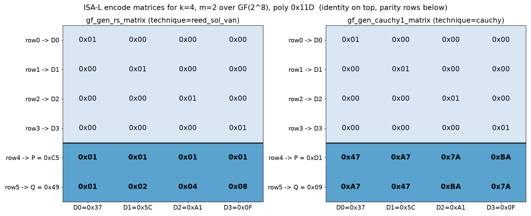
Why Ceph imposes limits. The gf_gen_rs_matrix matrix is not a "real" Vandermonde: identity rows have been placed on top of it, and it is not guaranteed to be MDS for every (k, m). ISA-L itself has the tool gen_rs_matrix_limits.c for finding the limits. Ceph applies these limits in ErasureCodeIsaDefault::parse: k ≤ 32 and m ≤ 32 (MAX_K and MAX_M). For Vandermonde, if m > 4, or m = 4 and k > 21, it logs a warning and changes the technique to cauchy automatically. That is, the stored profile is changed. A separate simulation (removing every combination of m rows and testing whether the remaining k×k matrix is invertible) found no singular submatrix for 4+2, 6+3, 8+3, 8+4, 10+4 and 12+4 (for example, 1001 combinations for 10+4), which is consistent with these limits.
27-10 decode with the matrix inverse: a complete byte-by-byte example#
Source in code: isa-l/erasure_code/ec_base.c :: gf_invert_matrix; src/erasure-code/isa/ErasureCodeIsa.cc :: ErasureCodeIsaDefault::isa_decode
Complexity: inverse O(k³) GF multiplications per failure pattern (cached in an LRU), then O(k·e·L) for e lost shards
pseudocode
B = the generator-matrix rows of the k chosen healthy shards
Binv = gf_invert_matrix(B)            # Gauss-Jordan: pivot, multiply the row by gf_inv, eliminate with ⊕
for each lost data shard i: c_i = row i of Binv
for each lost parity shard p: c_p = (row p of the generator matrix) × Binv
ec_init_tables(k, e, c, decode_tbls) ; ec_encode_data(L, k, e, decode_tbls, survivors, outputs)
Numerical example. We have the data [37 5C A1 0F] and the Vandermonde parities P = C5 and Q = 49. D1 and D3 are lost, and D0, D2, P and Q remain. First we remove the contribution of the known data:
- P' = P ⊕ D0 ⊕ D2 = C5 ⊕ 37 ⊕ A1 = 0x53, which equals D1 ⊕ D3.
- Q' = Q ⊕ D0 ⊕ 4·D2 = 49 ⊕ 37 ⊕ BE = 0xC0, which equals 2·D1 ⊕ 8·D3.
Eliminating D1: Q' ⊕ 2·P' = (8 ⊕ 2)·D3 = 0x0A·D3. We have 2·P' = 0xA6 and Q' ⊕ 0xA6 = 0x66. So D3 = 0x66 · inv(0x0A) = 0x66 · 0xDD = 0x0F and D1 = P' ⊕ D3 = 0x5C. The inverse matrix that gf_invert_matrix builds for the rows {0, 2, P, Q} has the row [7A F4 A7 DD] for D3 and the row [7B F5 A6 DD] for D1. Multiplying them by [37 A1 C5 49] gives the same two numbers.
27-11 Parity update with a delta (Tentacle)#
In the old EC, a partial write reads the whole stripe (the read-modify-write section). The optimized EC path in Tentacle, for plugins that declare the FLAG_EC_PLUGIN_PARITY_DELTA_OPTIMIZATION flag, uses the linearity of the code. Changing one data shard changes the parities only by that column's coefficient times the delta.
Source in code: src/erasure-code/isa/ErasureCodeIsa.cc :: ErasureCodeIsaDefault::encode_delta, apply_delta; isa-l :: ec_encode_data_update
Complexity: O(m·L) instead of O(k·m·L); reading 1 + m extents instead of k extents
pseudocode
encode_delta(old, new):  Δ = old ⊕ new                    # isa_xor with two vectors
apply_delta(in = {i: Δ_i, p: P_p}, out):
    for each data shard i with a delta:
        for each parity p:
            if m == 1:  P_p ^= Δ_i                          # the column is all 1
            else: ec_encode_data_update(L, k, 1, i, tbls + 32·k·(p−k), Δ_i, &P_p)
                  # P_p ^= a[p][i]·Δ_i
Numerical example. D1 changes from 0x5C to 0xA5, so Δ = 0x5C ⊕ 0xA5 = 0xF9. In Vandermonde the column-1 coefficients for P and Q are 1 and 2: P_new = C5 ⊕ F9 = 0x3C and Q_new = 49 ⊕ 2·F9 = 49 ⊕ EF = 0xA6. A full computation from scratch with the new data also gives exactly 3C and A6. In Cauchy the column-1 coefficients are A7 and 47, and the result is 0x17 and 0x70, which also matches the full computation. For a 4K write in 8+3, the old path needed 8 reads of 4K (or the whole stripe), while the delta path has 1 + 3 = 4 reads and 4 writes.
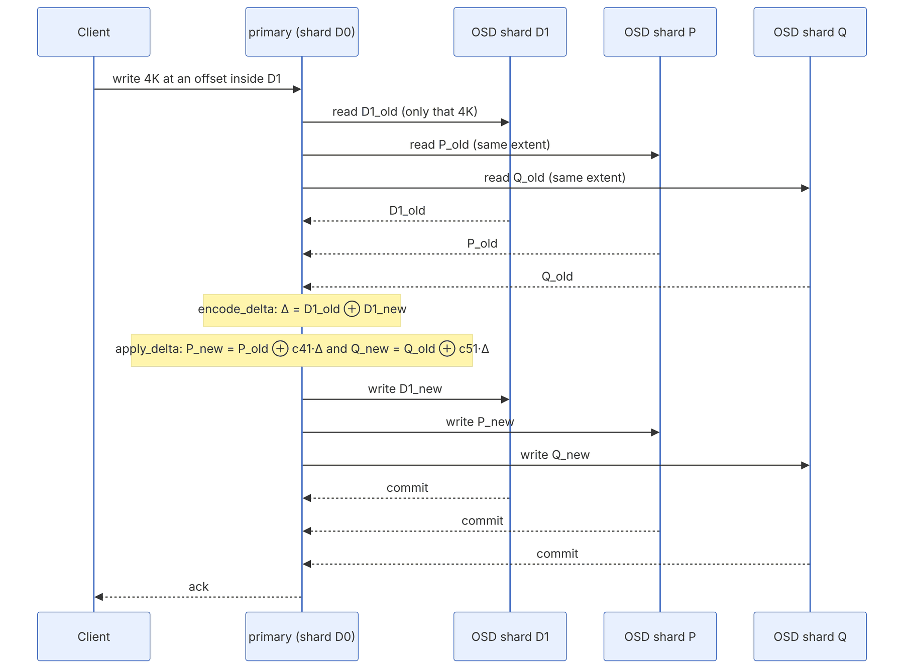
The delta is correct only if the old value that was read is exactly the value the current parity was built from. If a shard is inconsistent (for example after a half-finished error), the delta propagates the error. That is why deep scrub in EC pools (chapter 32) and the crc of each shard (the crc section of this chapter) become more important.
27-12 LRC: from k, m and l to the layer strings#
Source in code: src/erasure-code/lrc/ErasureCodeLrc.cc :: ErasureCodeLrc::parse_kml
Complexity: O(k+m) to build the strings; local repair reads l instead of k
pseudocode
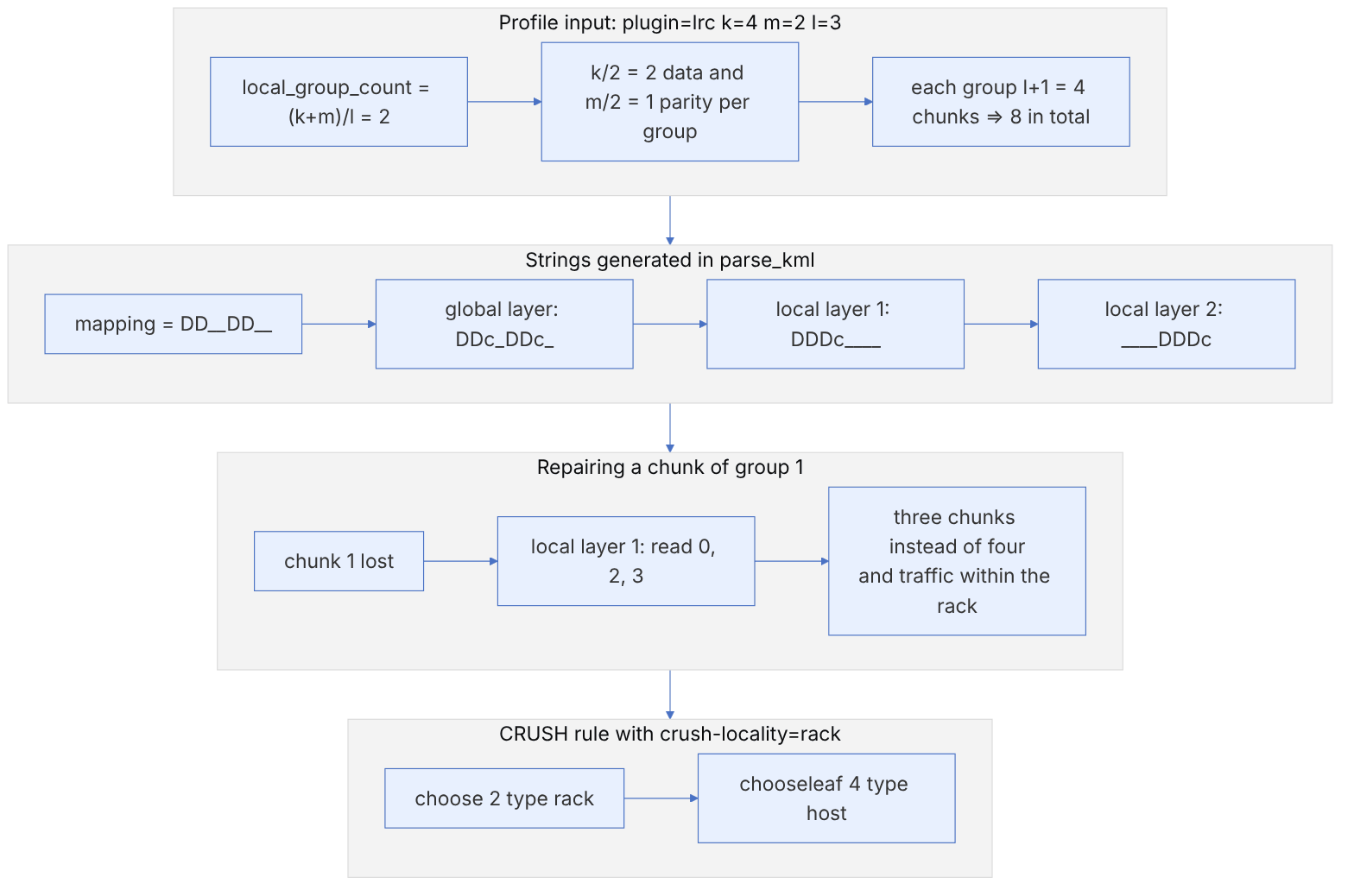
require (k+m) % l == 0 ; g = (k+m)/l ; require k % g == 0 and m % g == 0
mapping = repeat g: 'D'×(k/g) + '_'×(m/g) + '_'
global  = repeat g: 'D'×(k/g) + 'c'×(m/g) + '_'
local_i = for j < g: (i==j) ? 'D'×l + 'c' : '_'×(l+1)
if crush-locality: steps = [choose g type locality, chooseleaf (l+1) type failure-domain]
Numerical example. With k=4, m=2 and l=3: g = 6/3 = 2, and each group has 2 data chunks, 1 global parity and 1 local parity. The total number of chunks is 4 + 2 + 2 = 8. The result: mapping = DD__DD__, the global layer DDc_DDc_ and the local layers DDDc____ and ____DDDc. The space overhead is 8/4 = 2 times (versus 1.5 for a plain 4+2). In return, repairing one chunk needs only 3 reads from the same group instead of 4.
27-13 Clay: which sub-chunks are read for repair#
Source in code: src/erasure-code/clay/ErasureCodeClay.cc :: ErasureCodeClay::parse, get_repair_subchunks, get_repair_sub_chunk_count
Complexity: O(qʸ) extents for a lost node in row y; traffic of d·(sub_chunk_no/q) sub-chunks
pseudocode
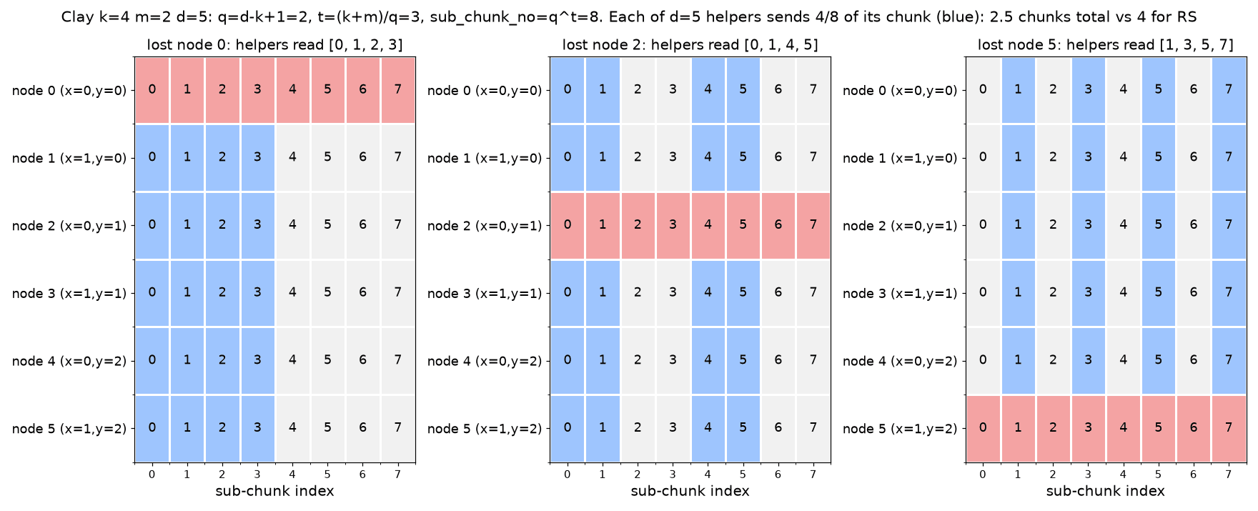
q = d − k + 1 ; nu = (k+m) % q ? q − (k+m) % q : 0
t = (k+m+nu)/q ; sub_chunk_no = q^t
get_repair_subchunks(lost):
    y = lost / q ; x = lost % q
    seq = q^(t−1−y) ; num = q^y ; idx = x·seq
    repeat num times: emit [idx, idx+seq) ; idx += q·seq
Numerical example. k=4, m=2, d=5 ⇒ q = 2, nu = 0, t = 3 and sub_chunk_no = 8. For node 0 (x=0, y=0): seq = 4 and num = 1, so sub-chunks 0 to 3. For node 2 (x=0, y=1): seq = 2 and num = 2, so {0, 1, 4, 5}. For node 5 (x=1, y=2): seq = 1 and num = 4, so {1, 3, 5, 7}. Each of the 5 helpers sends half of its chunk, that is 2.5 chunks versus 4 chunks in RS. A four-megabyte chunk is repaired with 2.5 × 4 = 10 MiB instead of 16 MiB.
In Clay, because the reads are split into small extents (sub_chunk_no of them), stripe_unit must be large enough for each sub-chunk to be at least a few kilobytes. If a chunk is only 4K and sub_chunk_no = 8, each sub-chunk is only 512 bytes (get_chunk_size rounds the actual chunk size to an alignment of sub_chunk_no·k).
27-14 Supplementary and up to date#
- Default plugin:
plugin=jerasurein Squid, andplugin=isain Tentacle and main (both withtechnique=reed_sol_van k=2 m=2). We checked this change in theglobal.yaml.incode of both branches. - Optimized EC: the main code has the
ECSwitchclass, described as a "temporary switch" between the old backend (ECBackendL) and the new one (ECBackend). According to the code's own comment, the old backend will be removed once there is full confidence in the new one. - EC and stretch clusters: work on supporting EC in stretch mode continues in the main branch. Read the release notes of the target release before using it.
27-15 Hands-on exercise#
- 1. Implement multiplication with 0x11D in Python and reproduce this chapter's multiplication table. Then solve a decode with two failures for another pattern (for example D0 and P1).
- 2. With
ceph_erasure_code_benchmark(in the test package), compare the encode speed of the isa and jerasure plugins for k=8 and m=3 on your server. - 3. On a test EC pool, with and without
allow_ec_optimizations, run fio with 4K random writes and compare IOPS and latency. - 4. Compute the CLAY repair bandwidth for (k=6, m=3, d=8) and compare it with RS.
27-16 Review questions#
- 1. Why are addition and subtraction in both XOR?
- 2. How is 0x56 × 0x04 computed in with 0x11D?
- 3. What is an MDS code, and why is ISA-L's simple Vandermonde not always MDS?
- 4. Under what conditions does Ceph switch to cauchy automatically?
- 5. In this chapter's example, how were P0 and P1 obtained?
- 6. Why are the decode coefficients cached?
- 7. How does PSHUFB make multiplication by a constant fast?
- 8. What is the parity delta, and why is it correct?
- 9. What is the default stripe_unit in an optimized pool, and why?
- 10. What is the CLAY repair bandwidth with k=8, m=4 and d=11, and what does it cost?
Answers to these questions are in Appendix E: Answers to Review Questions. Answers to this chapter's questions →
27-17 Sources for this chapter#
- Erasure code documentation
https://docs.ceph.com/en/latest/rados/operations/erasure-code/ - Profiles
https://docs.ceph.com/en/latest/rados/operations/erasure-code-profile/ - The CLAY plugin
https://docs.ceph.com/en/latest/rados/operations/erasure-code-clay/ - The LRC plugin
https://docs.ceph.com/en/latest/rados/operations/erasure-code-lrc/ - The SHEC plugin
https://docs.ceph.com/en/latest/rados/operations/erasure-code-shec/ - ErasureCodeIsa.cc
https://github.com/ceph/ceph/blob/main/src/erasure-code/isa/ErasureCodeIsa.cc - ISA-L ec_base.c
https://github.com/intel/isa-l/blob/master/erasure_code/ec_base.c - The Clay codes paper (FAST 2018
https://www.usenix.org/conference/fast18/presentation/vajha - Reed-Solomon tutorial (Plank
https://web.eecs.utk.edu/~jplank/plank/papers/CS-96-332.html