Storage Tiering: From Cache Tiering to Device Classes and Storage Classes
TL;DR this chapter in a few lines
- Cache tiering puts a fast pool in front of a base pool, but it has been deprecated since Reef.
- Remove an existing cache tier carefully: check the base pool's free space, flush and evict, then remove the overlay.
- Today's alternatives are device classes and CRUSH rules per pool, separating hot and cold data in the application, and RGW storage classes with lifecycle transitions.
- RocksDB data already spreads between fast and slow devices inside BlueStore.
16-1 Before you start#
16-1-1 What questions does this chapter answer?#
Every large cluster sooner or later faces this question: how do we keep hot data on fast, expensive media and cold data on cheap, high-capacity media? For years Ceph had an "official" answer to this question: Cache Tiering. Today the situation is different. The official documentation states explicitly that cache tiering was deprecated in Reef, has long had no maintainer, and may be removed in a future release without notice; no new cache tiers should be built, and existing deployments should migrate as soon as possible. This chapter covers both sides of the coin:
- How did cache tiering work, and why did it reduce performance for most workloads?
- With what algorithm did the tier agent inside the OSD flush and evict?
- If you still have a cache tier, how do you remove it safely?
- What are today's alternatives: device classes and CRUSH rules, block.db on NVMe, and storage classes and lifecycle in RGW?
16-2 Cache Tiering: architecture#
16-2-1 The overlay and the cache pool#
In cache tiering, a fast pool (the cache) sits in front of a base (backing) pool. With set-overlay, the OSDMap points the base pool's read_tier and write_tier fields at the cache pool. The client's Objecter sees these fields and transparently sends requests to the cache pool; the client does not need to know anything about the cache.
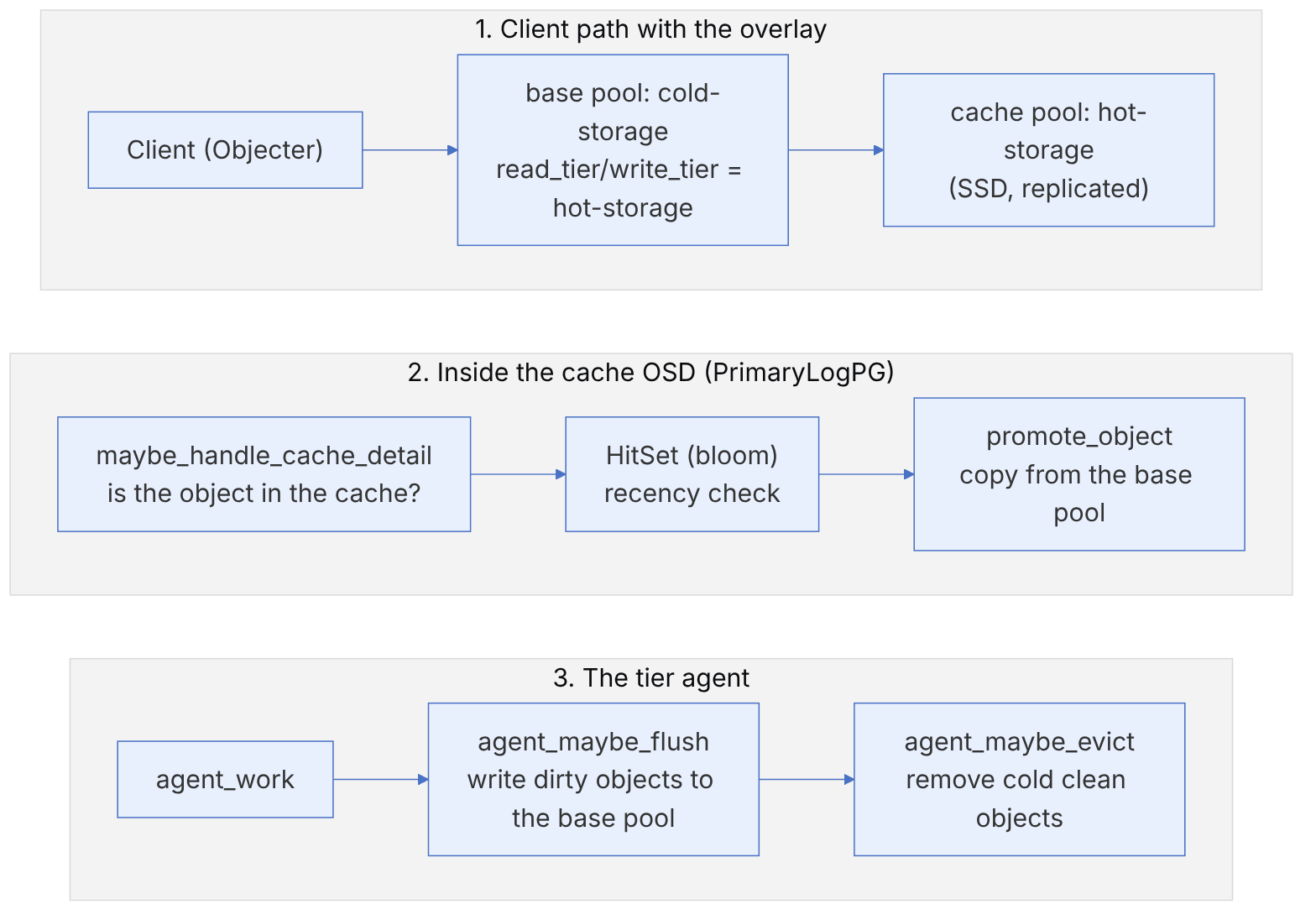
# only for understanding or a lab; do not build a new cache tier in a production cluster
ceph osd tier add cold-storage hot-storage
ceph osd tier cache-mode hot-storage writeback
ceph osd tier set-overlay cold-storage hot-storage
ceph osd pool set hot-storage hit_set_type bloom
ceph osd pool set hot-storage hit_set_count 12
ceph osd pool set hot-storage hit_set_period 14400
ceph osd pool set hot-storage target_max_bytes 1099511627776| Cache mode | Behaviour |
|---|---|
| writeback | Writes go to the cache and are acked immediately; the agent flushes later; reads are promoted |
| readproxy | Objects in the cache are used; missing objects are proxied from the base without promotion |
| readonly | Promotion only on reads; writes go straight to the base; cached data may be stale |
| proxy | All operations are proxied to the base; used for draining a writeback cache |
| none | The cache is completely disabled |
readonly mode does not guarantee consistency: after a write to the base pool, the old version in the cache may still be read. It was only suitable for immutable data.
16-2-2 HitSet: which object is hot?#
To decide on promotion, the cache OSD must know whether an object has been accessed recently. Every hit_set_period seconds, each PG builds a HitSet: the set of objects accessed in that interval. The recommended type is bloom (src/osd/BloomHitSet.h): a Bloom filter with low memory use and a controlled false-positive probability. The other types, explicit_hash and explicit_object, use more memory. hit_set_count is the number of HitSets kept, and min_read_recency_for_promote is the number of recent HitSets in which an object must have been seen to be promoted on a read; a value of 0 means always promote.
pseudocode: the promotion decision (this book's summary of maybe_handle_cache_detail)
  if object in cache pool:            serve locally
  elif mode == writeback/readproxy:
      recent = count(h in last min_read_recency HitSets if obj in h)
      if recent >= min_read_recency_for_promote:  promote_object(obj)  # copy from the base
else: proxy_read(obj) # read directly from the baseHitSets themselves are stored as hidden objects in the same cache PG (hit_set_persist() in PrimaryLogPG.cc) and trimmed with hit_set_trim(). This means the cache has extra I/O just for tracking hotness. Each promotion is also a read from the base pool plus a write to the cache; if the access pattern is scattered (most RBD workloads), the cache is constantly promoting and evicting, and performance becomes worse than a pool with no cache at all. The official documentation says exactly this: cache tiering reduces performance for most workloads and is only effective when accesses concentrate on a small set of objects (for example RGW reading mostly freshly written objects).
16-3 Inside the code: the tier agent#
16-3-1 agent_choose_mode: measuring fullness and dirtiness#
The tier agent is enabled in each cache PG with agent_setup(), and the OSD runs agent_work() on the active PGs in a separate thread (the maximum concurrent operations are controlled by osd_agent_max_ops, whose default in current code is 4). The main decision is made in PrimaryLogPG::agent_choose_mode(). The interesting point is that the whole-pool targets (for example target_max_bytes) are turned into each PG's share with a "divisor": pg_pool_t::get_pg_num_divisor() returns the number of PGs, accounting for an unfinished split (when pg_num is not a power of 2). All ratios are computed in micro units (millionths) with integers to avoid floating point.
pseudocode: agent_choose_mode (this book's rewrite from PrimaryLogPG.cc)
  divisor   = pool.get_pg_num_divisor(pgid)         # this PG's share of the pool target
  avg_size  = user_bytes / user_objects
  dirty_µ   = dirty_objs * avg_size * 1e6 / (target_max_bytes / divisor)
  full_µ    = user_objs  * avg_size * 1e6 / (target_max_bytes / divisor)
  if target_max_objects:                            # whichever is larger
      dirty_µ = max(dirty_µ, dirty_objs * 1e6 / (target_max_objects / divisor))
      full_µ  = max(full_µ,  user_objs  * 1e6 / (target_max_objects / divisor))

  slop = target * osd_agent_slop                    # hysteresis (default 0.02)
  target' = target + slop  if currently IDLE  else target - slop

  flush_mode = HIGH if dirty_µ > dirty_high' else LOW if dirty_µ > dirty' else IDLE
  if   full_µ > 1e6:        evict_mode = FULL; effort = 1e6     # evict every clean object
  elif full_µ > full':      evict_mode = SOME
      effort = max((full_µ - full') * 1e6 / (1e6 - full'), osd_agent_min_evict_effort)
      effort = quantize(effort, osd_agent_quantize_effort)   # less reshuffling in the agent queue
  else:                     evict_mode = IDLE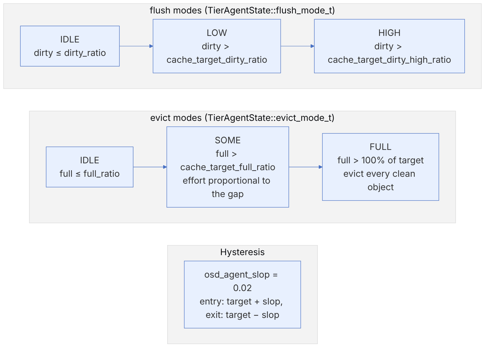
16-3-2 Choosing a victim: object temperature#
In SOME mode, agent_maybe_evict() estimates the "temperature" of each clean object with agent_estimate_temp() from the recent HitSets (for each HitSet containing the object, the weight pool.info.get_grade(i) is added; the weights decrease for older HitSets according to hit_set_grade_decay_rate, and an object in the current HitSet gets the maximum temperature) and puts it into a histogram (temp_hist). It then compares the object's position in the temperature distribution (get_position_micro) with evict_effort: the design intent is that hot objects are kept, but the actual condition in main's code is inverted (see the section "Temperature in numbers"). So eviction is not an exact LRU but statistical sampling over temperature, with a low memory cost.
pseudocode: agent_maybe_evict (summary)
  if obj dirty or in use or age < cache_min_evict_age: skip
  if evict_mode != FULL:
      temp = estimate_temp(obj, hitsets)             # weighted sum of presence in HitSets
      hist.add(temp); (lower, upper) = hist.position_µ(temp)
      if 1e6 - upper >= evict_effort: keep           # the code's literal condition; its meaning is examined in "Temperature in numbers"
evict(obj) # remove from the cache; the valid copy is in the base poolFlushing happens in agent_maybe_flush() and start_flush(): the dirty object (with its snapshots) is written to the base pool with a copy-from operation, and after confirmation the dirty flag is cleared. cache_min_flush_age prevents flushing an object that was just written. If the cache reaches target_max_bytes or target_max_objects and the agent cannot flush and evict enough, the OSD blocks client requests; this was one of the most common causes of outages in clusters with a cache.
If neither target_max_bytes nor target_max_objects is set, the fullness ratios compute as zero and the agent never evicts based on fullness; the cache grows until the OSDs fill up. You also saw in the pseudocode above that fullness is only computed when these targets are set.
16-4 Migration: safely removing a cache tier#

# 1. current state
ceph osd pool ls detail | grep -E "tier|cache_mode|read_tier|write_tier"
ceph df detail
# 2. stop promotion and writes into the cache
ceph osd tier cache-mode hot-storage proxy
# 3. drain (may take hours; monitor progress)
rados -p hot-storage cache-flush-evict-all
rados -p hot-storage ls | head
# 4. remove the overlay and the tier
ceph osd tier remove-overlay cold-storage
ceph osd tier remove cold-storage hot-storageBefore starting, check the free capacity of the base pool: every dirty object must be written there. If the base pool is EC on HDD, a bulk flush creates a heavy load; do it during quiet hours and monitor ceph -s and client latency.
For old upgrades (14.2.6 to 14.2.7), the official documentation recorded a case of unfound objects after restarting OSDs in a cache pool. If you see something like this after an upgrade or restart, check ceph pg <pgid> list_unfound before taking any action, and follow the guidance on that page.
16-4-1 If the base pool is EC#
The historical reason for many cache tiers was that before Luminous, EC pools did not support overwrites, and RBD or CephFS could not work on them directly. Today, with allow_ec_overwrites (and in Tentacle, the FastEC optimizations; chapter 13), this limitation is gone: metadata goes in a replicated pool and data in an EC pool (rbd create --data-pool, or adding an EC data pool to CephFS).
16-5 Tiering at the byte level: storage classes and lifecycle in RGW#
In the previous sections we saw that cache tiering has been deprecated since Reef (the warning at the top of the cache-tiering.rst document) and what today's alternatives are: device classes, separate pools for data and metadata, and storage classes in RGW. This section shows what actually changes in RADOS when an S3 object "moves between tiers".
16-5-1 The layout of an RGW object#
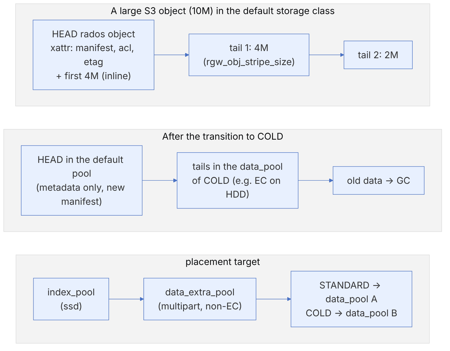
The manifest (in the xattr named user.rgw.manifest) maps the logical object to RADOS objects: the head size, the stripe size, the prefix of the tail objects and their naming rules. This explains why a transition looks "cheap" but is in fact a full copy of the data: RGW reads the data from the old tails, writes it into the new class's pool, updates the manifest and gives the old objects to GC for deletion. The bandwidth of lifecycle is the cluster's bandwidth.
| Option / attribute | Value (main) | Effect |
|---|---|---|
rgw_max_chunk_size | 4_M | Size of the head chunk and RGW's read/write unit |
rgw_obj_stripe_size | 4_M | Size of the tail objects |
--placement-inline-data | true (default) | The first data goes in the head; per the documentation, inlining happens only in the default class |
data_extra_pool | e.g. default.rgw.buckets.non-ec | Metadata of unfinished multipart uploads; must be replicated (omap) |
index_pool | e.g. default.rgw.buckets.index | Bucket index (omap only); the best place for SSD or NVMe |
According to the placement.rst document, if BlueStore's DB is on a faster device than the bucket data, turning off inlining (--placement-inline-data=false) can make client deletes faster, because on DELETE RGW no longer has to touch the slow device synchronously, and the data is removed later by GC. The trade-off is an extra round trip for reading and writing small objects.
16-5-2 How does lifecycle run?#
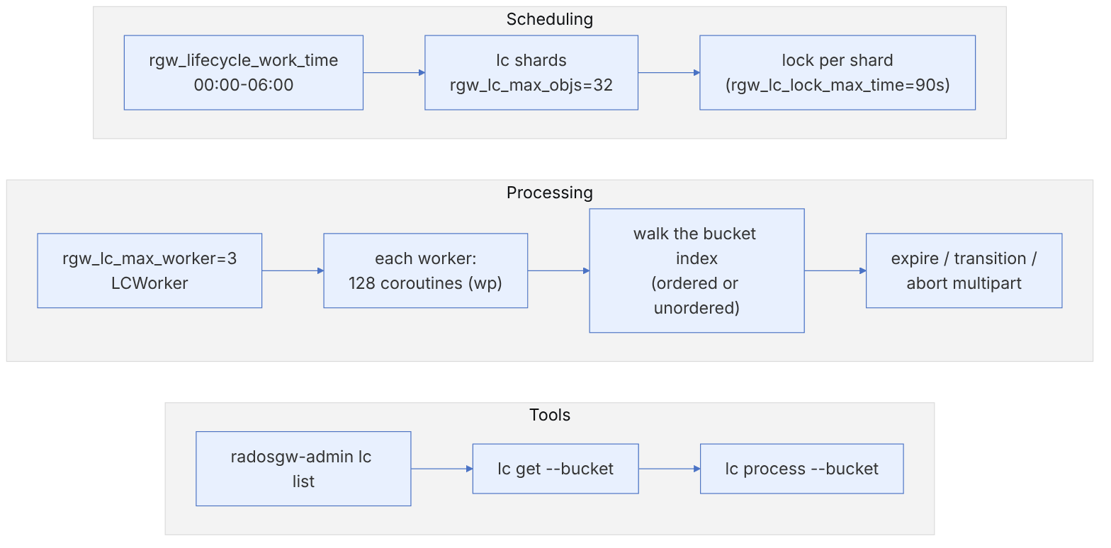
radosgw-admin lc list                          # state of each bucket: UNINITIAL / PROCESSING / COMPLETE
radosgw-admin lc get --bucket photos
radosgw-admin lc process --bucket photos       # manual run (outside the window)
radosgw-admin gc list --include-all | head
ceph config set client.rgw rgw_lifecycle_work_time "00:00-23:59" # for testing onlyCapacity calculation: with 3 workers and 128 coroutines, up to about 384 objects are processed concurrently at any moment. If 50 terabytes must move from STANDARD to COLD every night and the work window is 6 hours, the cluster must sustain about 50 TB / 21600 s ≈ 2.3 GB/s of reads and the same amount of writes (plus EC or replication overhead) on top of the normal load. Otherwise lifecycle falls behind every night and its queue grows. Compute this number before defining transition rules.
16-5-3 Tiering inside an OSD#
Tiering is not only between pools. An OSD with block.db and block.wal devices has three tiers. Chapter 25 showed that BlueFS spreads RocksDB levels across WAL, DB and the slow device with the use_some_extra policy. Chapter 24 showed that deferred writes smaller than bluestore_prefer_deferred_size (64K on HDD) are first written to RocksDB's WAL (that is, on the fast device) and moved to the HDD later. This is effectively a small write-back cache for small writes on HDD, without the complexities of cache tiering. Chapter 28 also showed that device classes, with separate shadow trees, guarantee that adding a device to one class moves no data in the pools of another class.
| Tier | Mechanism | Chapter |
|---|---|---|
| PG→device | device class + CRUSH rule | 8 and 28 |
| RGW metadata | index_pool and data_extra_pool on SSD | 4 and this chapter |
| Cold data | storage class and lifecycle transition | this chapter |
| OSD metadata | block.db and block.wal (BlueFS) | 12, 24 and 25 |
| Small writes on HDD | deferred writes | 12 and 24 |
| RBD metadata | a separate data pool (--data-pool) on EC | 2 and 13 |
16-6 Tiering in numbers: six algorithms from the code#
This section examines the tiering mechanisms described above with code and numbers. Three algorithms concern cache tiering (deprecated, but still in main's code), two concern lifecycle in RGW, and one concerns placing RocksDB data between the fast and slow devices inside an OSD.
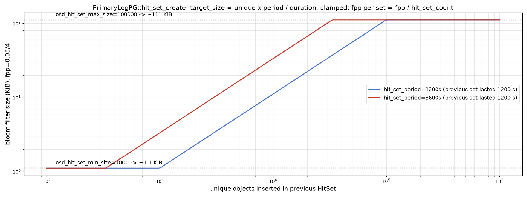
16-6-1 HitSet size#
Source in code: src/osd/PrimaryLogPG.cc :: PrimaryLogPG::hit_set_create; src/osd/BloomHitSet.h :: BloomHitSet
Complexity: O(1) to determine the size; memory −n·ln(p)/(ln 2)² bits
pseudocode
p = fpp_pool / hit_set_count ; if p ≤ 0: p = 0.01
if target_size == 0 and a previous hit_set exists:
    target_size = unique_inserts(previous) × hit_set_period / actual duration of previous
target_size = clamp(target_size, osd_hit_set_min_size = 1000, osd_hit_set_max_size = 100000)
seed = now.sec ; BloomHitSet(target_size, p, seed)
Numerical example. With the osd_tier_default_cache_* defaults that ceph osd tier add-cache applies (bloom, hit_set_count = 4, hit_set_period = 1200 s) and osd_pool_default_hit_set_bloom_fpp = 0.05, the false-positive rate of each set is 0.05/4 = 0.0125. If the previous HitSet saw 30000 unique objects in 1200 seconds, target_size = 30000, and the filter is about bits (about 33 KiB) with 6 hash functions. The cap of 100000 objects gives a filter of about 111 KiB, and the floor of 1000 about 1.1 KiB. The reason for dividing the fpp by the number of sets is that temperature comes from summing presence across several sets, and each set's error adds up.
16-6-2 Temperature in numbers#
Source in code: src/osd/osd_types.h :: pg_pool_t::calc_grade_table, get_grade; src/osd/PrimaryLogPG.cc :: agent_estimate_temp, agent_maybe_evict; src/common/histogram.h :: pow2_hist_t::get_position_micro
Complexity: O(hit_set_count) per object; power-of-two histogram O(log temp)
pseudocode
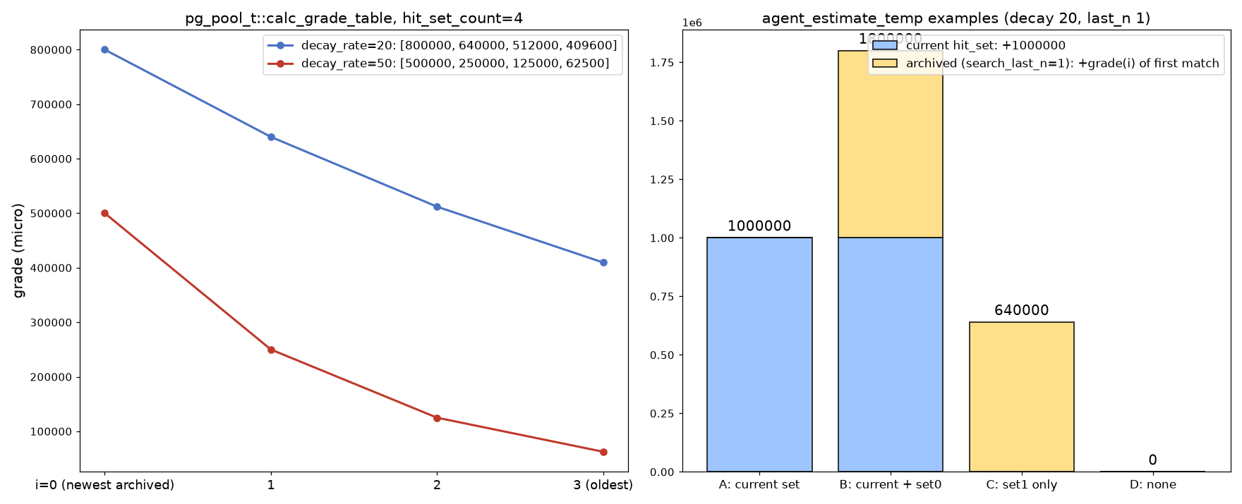
calc_grade_table: v = 10^6 ; for i < count: v = v × (1 − decay/100) ; grade[i] = v
estimate_temp(o): t = (o ∈ current) ? 10^6 : 0
    for i, set in archived (newest to oldest) while last_n > 0: if o ∈ set: t += grade[i] ; last_n−−
agent_maybe_evict (SOME mode):
    hist.add(t) ; (lower, upper) = hist.position_µ(t)   # upper = share of objects with bin ≤ bin(t)
    if 10^6 − upper ≥ evict_effort: keep  else: evict   # main's literal condition; inverted relative to the intent "evict the cold"
Numerical example. With the osd_tier_default_cache_* defaults (decay_rate = 20, search_last_n = 1), the grade table is 800000, 640000, 512000 and 409600. Four sample objects:
- A is only in the current set: temperature 1000000.
- B is in the current set and in set 0: 1800000.
- C is only in set 1: 640000.
- D is in no set: 0.
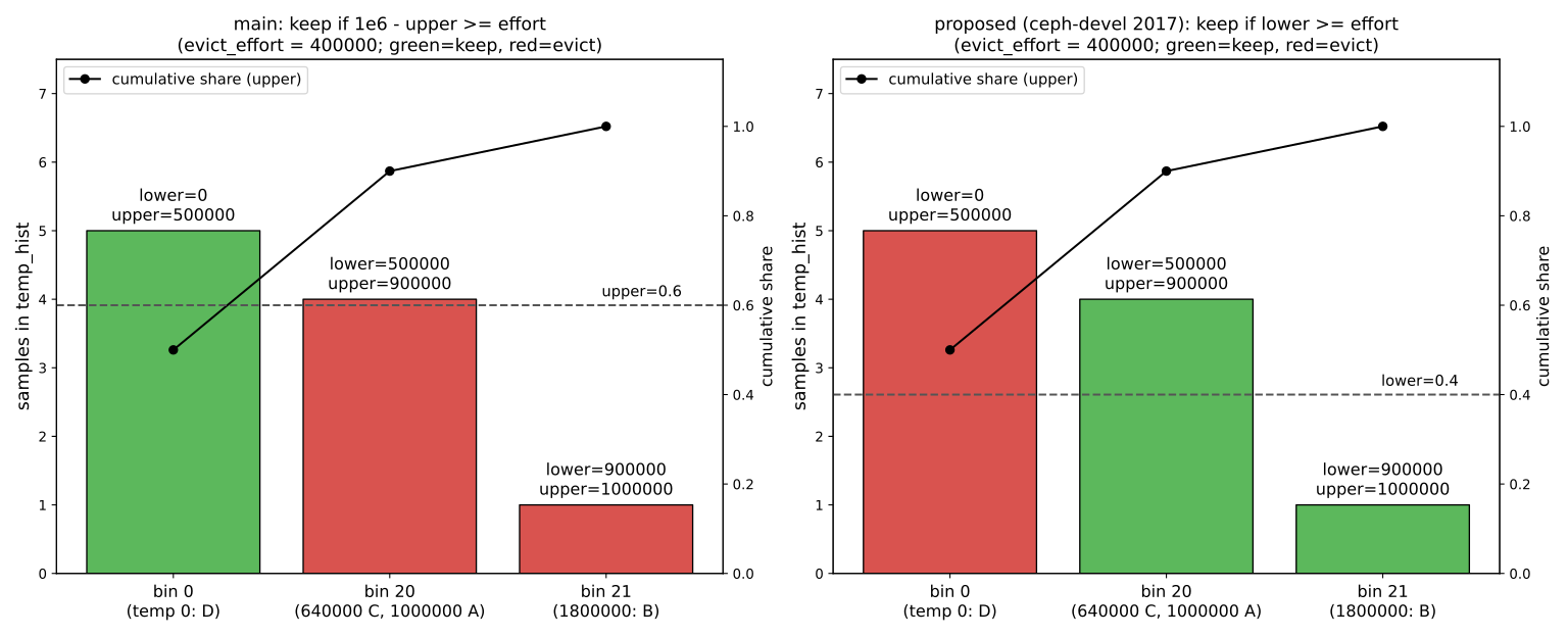
Now the meaning of the code's condition: get_position_micro sets upper to the share of objects whose power-of-two temperature bin (cbits(temp), that is, the index of the highest set bit) is less than or equal to this object's bin, and lower to the share of objects in smaller bins. Let us build a ten-sample histogram: five samples with temperature 0 (bin 0), two samples at 640000 and two at 1000000 (both bin 20), and one sample at 1800000 (bin 21). With evict_effort = 400000 the result is:
| Object | Temperature | bin | lower | upper | main's decision | Decision with the proposed fix (lower ≥ effort ⇒ keep) | |
|---|---|---|---|---|---|---|---|
| D | 0 | 0 | 0 | 500000 | 500000 | keeps | evicts |
| C | 640000 | 20 | 500000 | 900000 | 100000 | evicts | keeps |
| A | 1000000 | 20 | 500000 | 900000 | 100000 | evicts | keeps |
| B | 1800000 | 21 | 900000 | 1000000 | 0 | evicts | keeps |
These numbers were obtained with a Python reimplementation of pow2_hist_t::get_position_micro. So main's condition really is inverted: the coldest object (D) stays and the hot ones are evicted. This inversion has a documented history. Before Jewel, the agent used "time since last access" (atime) instead of temperature, which is larger for cold data, and the condition 1000000 − atime_upper ≥ evict_effort ⇒ keep was correct with that meaning. PR number 4737 (branch wip-temp-based-object-eviction) changed the metric to temperature, which is smaller for cold data, but only renamed the variable in the condition. In November 2017 this exact issue was reported on the ceph-devel list (thread "About the "temperature histogram" of tier-agent"), and Sage Weil referred it to that PR's authors for review. It was proposed to change the condition to temp_upper ≥ evict_effort or temp_lower ≥ evict_effort, but in today's main code (checked in November 2026) the condition still has the same old form. In EVICT_MODE_FULL this condition is not executed at all, and every clean, eligible object is evicted; so the effect of the inversion is only seen in SOME mode. This is one more reason why cache tiering (deprecated since Reef) should not be chosen for new work.
16-6-3 evict_effort in numbers#
Source in code: src/osd/PrimaryLogPG.cc :: PrimaryLogPG::agent_choose_mode
Complexity: O(1) per PG per agent run
pseudocode
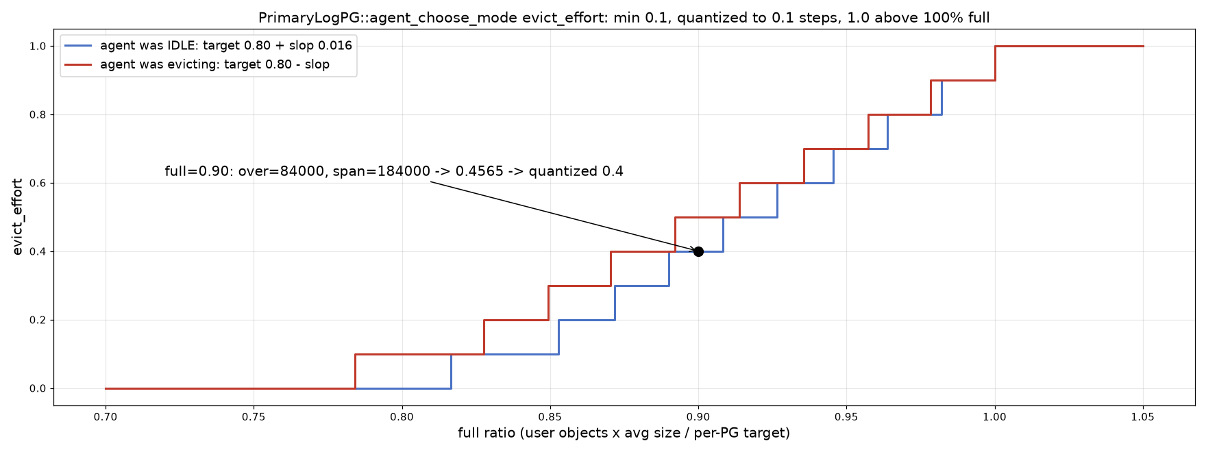
target = cache_target_full_ratio × 10^6 ; slop = target × osd_agent_slop (0.02)
target = (IDLE or restart) ? target + slop : target − slop        # hysteresis
if full_µ > 10^6: FULL ; effort = 10^6
elif full_µ > target: SOME
    effort = max((full_µ − target) × 10^6 / (10^6 − target), 0.1 × 10^6)
    effort −= effort % (0.1 × 10^6) ; effort = max(effort, 0.1 × 10^6)
Numerical example. cache_target_full_ratio = 0.8 (the default), so target = 800000 and slop = 16000. The agent starts from IDLE, so the threshold is 816000. With full = 0.90: over = 84000, span = 184000, and the raw effort is 456521, which rounds to 400000. When fullness returns to 0.80, the exit threshold is 784000. So the agent stays in SOME until full ≤ 0.784. The 3.2 percent gap between entry and exit prevents rapid back-and-forth. Rounding to steps of 0.1 also keeps the order of the agent queue in the OSD stable.
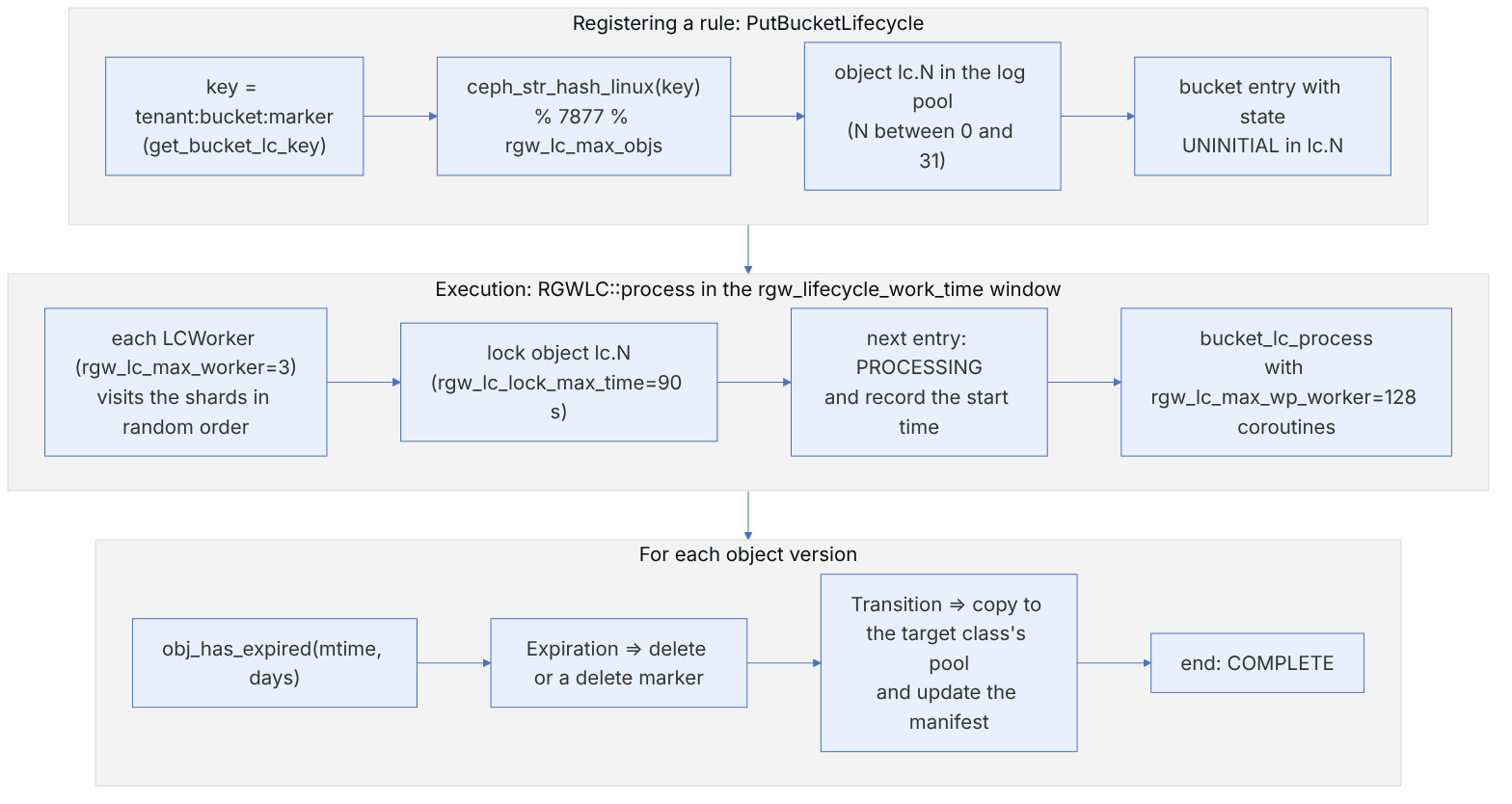
16-6-4 The lifecycle shard and choosing the lc.N object#
Source in code: src/rgw/rgw_lc.cc :: get_lc_index, get_bucket_lc_key, random_sequence, RGWLC::process; src/common/ceph_hash.cc :: ceph_str_hash_linux
Complexity: hash O(key length); each worker O(rgw_lc_max_objs) shards per round
pseudocode
key = tenant + ":" + bucket + ":" + marker
h = 0 ; for c in key: h = (h + (c ≪ 4) + (c ≫ 4)) × 11   (mod 2^32)
index = h % 7877 % min(rgw_lc_max_objs, 7877)    # default 32 ⇒ lc.0 .. lc.31
RGWLC::process(worker): for shard in shuffle(0..31):
    lock lc.shard (at most rgw_lc_lock_max_time = 90 s) ; mark the next entry PROCESSING ; unlock
    bucket_lc_process(bucket) with a pool of rgw_lc_max_wp_worker coroutines
Numerical example. A bucket's marker in RADOS is created at bucket creation by RGWRados::create_bucket_id, and its format is <zone id>.<instance id>.<counter>: the zone id (a UUID), the id of that radosgw's RADOS client instance, and an increasing counter. The marker below has the real format, but its UUID and two numbers are examples and do not come from a real cluster. For a bucket named photos, an empty tenant and the marker 3f6e1c2a-77b1-4e0b-9d2c-1a2b3c4d5e6f.4137.1, the key (which get_bucket_lc_key builds with the ":" separator) is :photos:3f6e…4137.1. ceph_str_hash_linux gives 2997460109. 2997460109 mod 7877 = 1668 and 1668 mod 32 = 4, so this bucket's entry is written in the object lc.4. The three workers (rgw_lc_max_worker) visit the shards in random order so that they do not all go to lc.0 at the same time. Because the hash is weak and there are only 32 shards, several large buckets may fall into one shard and be processed one after another. radosgw-admin lc list shows the state of each bucket.
16-6-5 On what day does an object expire?#
Source in code: src/rgw/rgw_lc.cc :: obj_has_expired; src/include/utime.h :: utime_t::round_to_day
Complexity: O(1) per object version
pseudocode
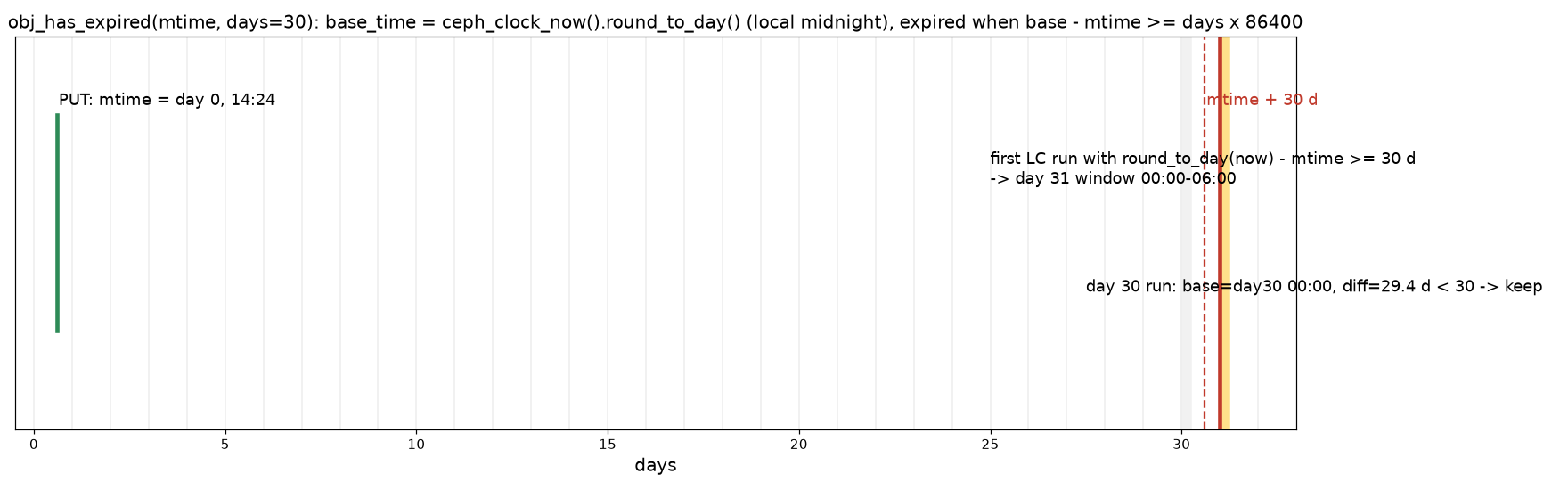
if rgw_lc_debug_interval ≤ 0:
    cmp = days × 86400 ; base = round_to_day(now)        # today's local midnight (localtime_r/mktime)
else: cmp = days × rgw_lc_debug_interval ; base = now     # test mode: each "day" is a few seconds
expired = (base − mtime) ≥ cmp ; expire_time = mtime + cmp
Numerical example. An object was written on day 0 at 14:24 and has an Expiration rule with Days = 30. The run on day 30: base = midnight of day 30, the gap is 29.4 days, less than 30, so it stays. The run on day 31: the gap is 30.4 days, so it is deleted. So the object effectively lives between 30.4 and 31.25 days (depending on when the worker runs in the window). Because base comes from the RGW server's local clock, two RGWs in different time zones may differ by a day. With rgw_lc_debug_interval = 10, each rule day is 10 seconds and Days = 30 means 300 seconds, which is useful for testing rules in a lab.
16-6-6 Placing RocksDB levels between the DB and the slow device#
Source in code: src/os/bluestore/BlueFS.h :: RocksDBBlueFSVolumeSelector (constructor, get_extra_level, get_hint_by_dir); src/os/bluestore/BlueStore.cc :: BlueStore::_open_bluefs (building the vselector)
Complexity: O(log_multiplier(DB/base)) for the level loop, once at mount
pseudocode
db_total = 0.95 × DB size ; L0 = write_buffer_size × max_write_buffer_number
if bluestore_volume_selection_reserved == 0:
    prev = L0 ; cur = base ; extra_level = 1
    loop: next = cur × mult ; extra_level++
          if db_total ≤ prev + cur + next:
              db_avail4slow = max(0, db_total − (prev + cur × reserved_factor)) ; break
          prev += cur ; cur = next
else: db_avail4slow = max(0, db_total − reserved) ; extra_level = 0
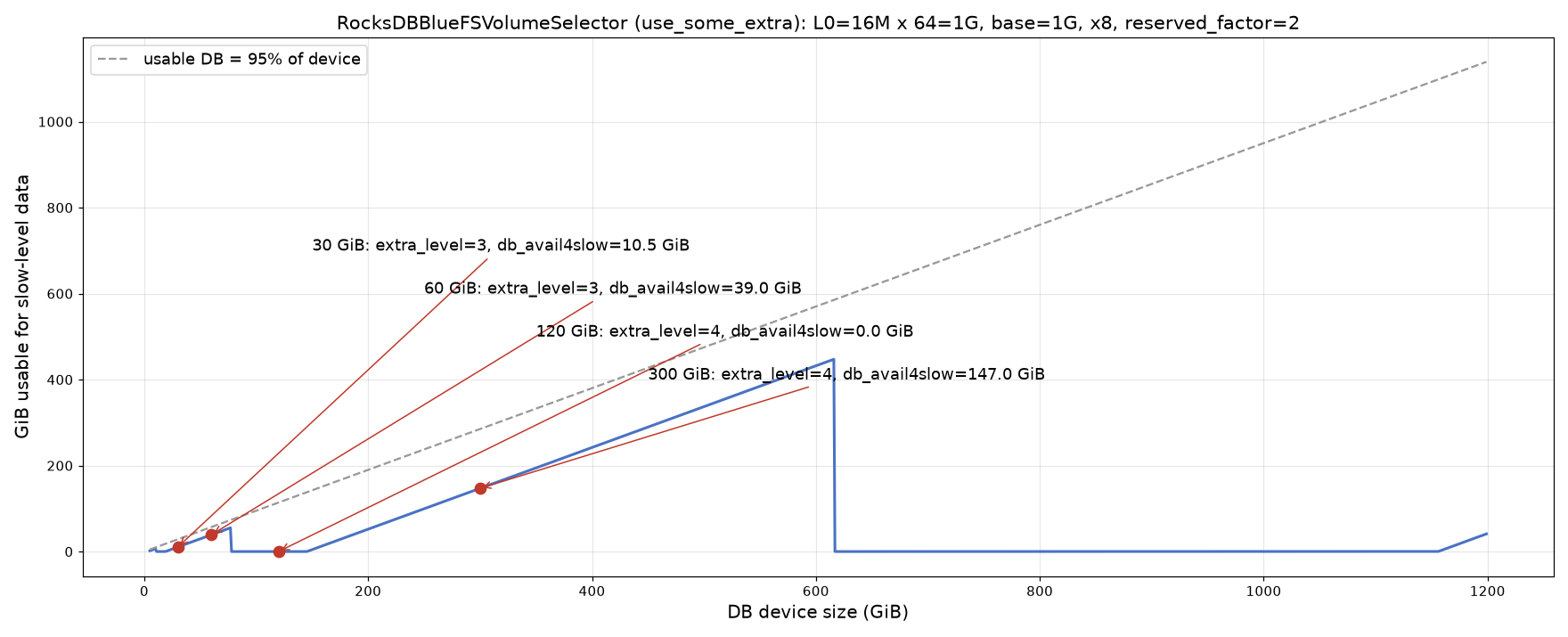
Numerical example (Ceph defaults: L0 = 16 MiB × 64 = 1 GiB, base = 1 GiB, mult = 8, reserved_factor = 2).
- A 30 GB DB (28.5 GiB usable): the loop stops at the threshold 2 + 8 + 64, and cur_threshold = 2 + 8×2 = 18, so 10.5 GiB remains on the DB for slow-level data.
- A 60 GB DB: 57 − 18 = 39 GiB.
- A 120 GB DB (114 GiB): the loop goes one level further (threshold 10 + 64 + 512). cur_threshold = 10 + 64×2 = 138 is larger than 114, so db_avail4slow = 0.
- A 300 GB DB: 285 − 138 = 147 GiB.
So a larger DB does not always give more extra space. Sizes that fall just after a level boundary benefit the least. This is the reason behind the old advice "make the DB 30, 300 or 3000 gigabytes". The fit_to_fast policy sets this calculation aside and fills up to 95% of the fast device.
This calculation only determines where BlueFS prefers to put the files of the higher levels. If the DB fills up, BlueFS still spills onto the slow device (spillover), and the BLUEFS_SPILLOVER warning appears in ceph health. ceph daemon osd.N bluefs stats shows the real distribution of each level across WAL, DB and SLOW.
16-7 Today's alternatives#
16-7-1 1. Device classes and a separate pool for each tier#
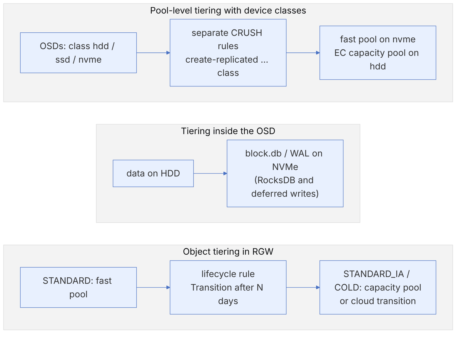
The simplest and most predictable method: separate hot and cold data at the application level and put each in a suitable pool. Since Luminous, each OSD has a device class (hdd, ssd, nvme or a custom name), and a CRUSH rule can select only the OSDs of one class.
ceph osd crush class ls
ceph osd crush rule create-replicated fast-rule default host nvme
ceph osd erasure-code-profile set cold-ec k=4 m=2 crush-failure-domain=host crush-device-class=hdd
ceph osd pool create vm-fast 128 128 replicated fast-rule
ceph osd pool create archive 256 256 erasure cold-ec
ceph osd pool set archive allow_ec_overwrites true
# RBD with metadata on the fast pool and data on EC
rbd create --size 1T --data-pool archive vm-fast/backup01Moving a pool to another tier takes only a CRUSH rule change: ceph osd pool set <pool> crush_rule fast-rule. Ceph moves the data with backfill; limit its effect on clients with osd_max_backfills and the mclock scheduler (chapter 21).
16-7-2 2. Tiering inside the OSD with BlueStore#
For HDD OSDs, placing block.db (RocksDB) and the WAL on NVMe gives the biggest effect for the least complexity: metadata, omap and small deferred writes (chapter 12; bluestore_prefer_deferred_size_hdd=64K) happen on fast media, and the HDD sees only large, sequential writes. In cephadm, with an OSD service specification:
service_type: osd
service_id: hdd-with-nvme-db
placement:
  host_pattern: 'stor-*'
spec:
  data_devices:
    rotational: 1
  db_devices:
    rotational: 0
16-7-3 3. Storage classes and lifecycle in RGW#
For object storage, the S3 pattern, that is storage classes and transitions with lifecycle, is the closest replacement for a "cache", with the important difference that the decisions are deterministic and auditable, not statistical.
radosgw-admin zonegroup placement add --rgw-zonegroup default \
    --placement-id default-placement --storage-class COLD
radosgw-admin zone placement add --rgw-zone default \
    --placement-id default-placement --storage-class COLD \
--data-pool default.rgw.cold.data --compression lz4{ "Rules": [ { "ID": "to-cold-after-30d", "Status": "Enabled",
"Filter": { "Prefix": "logs/" },
"Transitions": [ { "Days": 30, "StorageClass": "COLD" } ] } ] }aws --endpoint-url https://s3.example.internal s3api put-bucket-lifecycle-configuration \
--bucket app-logs --lifecycle-configuration file://lc.json
radosgw-admin lc listRGW also supports cloud transition: a storage class of type cloud-s3 that moves objects to an external S3 endpoint (the Cloud Transition page in the documentation). This is suitable for long-term archiving in another location.
16-7-4 4. Other tools#
- primary affinity: with
ceph osd primary-affinity <osd> <weight>you can lower the probability that slow OSDs become primary, so that more reads are served from the fast OSDs (in a replicated pool with mixed OSDs). - read balancer (since Reef): distributing primaries to balance the read load; the Read Balancer page in the documentation.
- Client-side caches: the librbd cache, librbd's persistent write-back cache (PWL), and fscache for kernel CephFS.
| Need | Recommended approach today |
|---|---|
| Latency-sensitive VMs | A replicated pool on nvme with a device class |
| Archive and backup | An EC pool on hdd, RBD with --data-pool |
| HDD OSDs with a mixed workload | block.db/WAL on NVMe |
| Object data with a known lifetime | Storage classes and lifecycle in RGW |
| Archiving outside the cluster | Cloud transition in RGW |
- Do not build a new cache tier; it is deprecated since Reef and may be removed without notice.
- Before upgrading a cluster with a cache tier, complete the migration.
- To remove a writeback tier: proxy, flush-evict-all, remove-overlay, remove.
- Do tiering at the pool and application level; the behaviour is predictable.
- For HDD OSDs, block.db on NVMe is the biggest cheap improvement.
16-8 Supplementary and up to date#
- From 2019 to today, the most important change in this area is the deprecation of cache tiering in Reef; the latest documentation still carries this warning.
- Overwrites in EC pools since Luminous, and FastEC in Tentacle, have removed the main historical reason for a cache tier in front of an EC pool.
- RGW storage classes, lifecycle and cloud transition are the official path for object tiering.
- The tier agent code (
agent_*inPrimaryLogPG.ccandTierAgentState.h) still exists in the main branch, but without a maintainer.
16-9 Hands-on exercise#
- 1. In a test cluster, build a writeback cache tier, apply a random load with
rados bench, and compare the latency with a pool without a cache. - 2. Set
target_max_bytessmall and follow the flush and evict mode transitions in the OSD log (level 20). - 3. Run the tier removal procedure completely and confirm that no object was lost.
- 4. Build two CRUSH rules with device classes and move a pool between tiers by changing crush_rule.
- 5. Build a COLD storage class in RGW and test the transition with a one-day lifecycle (for testing, set
rgw_lc_debug_intervalin the test environment). - 6. Read
agent_choose_modein the code and compute each PG's share for a pool with 128 PGs and a target_max_bytes of one terabyte.
16-10 Review questions#
- 1. What is the official status of cache tiering in current releases?
- 2. How does the overlay route a client request to the cache pool?
- 3. What advantage does a bloom-type HitSet have, and what does min_read_recency_for_promote do?
- 4. Why did cache tiering reduce performance for most RBD workloads?
- 5. How does the tier agent turn the whole-pool target into each PG's share?
- 6. What is the role of osd_agent_slop?
- 7. How does eviction in SOME mode choose a victim?
- 8. Write down the steps for removing a writeback cache tier.
- 9. What removed the historical reason for a cache tier in front of an EC pool?
- 10. What alternative is recommended for object data with a known lifetime?
Answers to these questions are in Appendix E: Answers to Review Questions. Answers to this chapter's questions →
16-11 Sources for this chapter#
- Cache Tiering (deprecation notice
https://docs.ceph.com/en/latest/rados/operations/cache-tiering/ - CRUSH maps and device classes
https://docs.ceph.com/en/latest/rados/operations/crush-map/ - Read balancer
https://docs.ceph.com/en/latest/rados/operations/read-balancer/ - RGW placement and storage classes
https://docs.ceph.com/en/latest/radosgw/placement/ - RGW cloud transition
https://docs.ceph.com/en/latest/radosgw/cloud-transition/ - Erasure code (overwrites
https://docs.ceph.com/en/latest/rados/operations/erasure-code/ - Source: src/osd/PrimaryLogPG.cc (agent_*, hit_set_*
https://github.com/ceph/ceph/blob/main/src/osd/PrimaryLogPG.cc - Source: src/osd/TierAgentState.h
https://github.com/ceph/ceph/blob/main/src/osd/TierAgentState.h - Source: src/osd/HitSet.h
https://github.com/ceph/ceph/blob/main/src/osd/HitSet.h - ceph-devel (2017-11), "About the "temperature histogram" of tier-agent"
https://www.spinics.net/lists/ceph-devel/msg39274.html