Ceph: A New Era — Architecture, Planning and Your First Cluster
TL;DR this chapter in a few lines
- Ceph is software-defined storage: block (RBD), object (RGW) and file (CephFS) interfaces all sit on one layer, RADOS, instead of RAID arrays.
- MONs hold the cluster maps, the MGR holds statistics and modules, and OSDs hold the data; CRUSH computes where an object lives, so there is no central lookup table.
- Planning decides success: workload, failure domain, network and MTU, fill ratio, and SSDs with power-loss protection for DB/WAL and MONs.
- cephadm is the official deployment tool: bootstrap one host, add hosts, and declare the desired services with
ceph orch apply.
1-1 Before you start#
1-1-1 What questions does this chapter answer?#
On the surface the first chapter is an "introduction", but in practice it builds the mental map on which the rest of the book rests. Every concept we meet in later chapters, from RBD and RGW to CRUSH, BlueStore and erasure coding, ultimately goes back to a few simple ideas introduced here: software-defined storage, the removal of a "central table of where data lives", and the intelligent distribution of responsibility across thousands of independent daemons. In this guide we try to answer these questions:
- Why does traditional storage built on RAID and dedicated arrays hit a dead end at today's scale, and exactly which pains does Ceph cure?
- Which layers and daemons make up the Ceph architecture, and what is each one responsible for?
- What path does an object take from the moment a client writes it until it is stored on three disks in three racks?
- Which questions must be answered before you buy hardware or build your first cluster?
- How do you build a real test cluster with cephadm, grow it and work with it?
1-1-2 Prerequisites and how to read#
This chapter assumes you are familiar with Linux, basic disk concepts (partitions, LVM, file systems) and networking (IP, subnets, MTU). Experience with containers (Podman or Docker) helps, because modern Ceph runs all of its daemons in containers. If you do not have a test cluster, the "Building the lab" section suggests a complete path with four virtual machines.
Many older Ceph tutorials were written against the Jewel and Luminous releases and use tools such as ceph-deploy and ceph-ansible for installation. Both tools have since been retired. In this book all examples are written with cephadm and current Ceph releases. Wherever behaviour differs between releases, we say so explicitly.
Throughout the text you will see several kinds of box:
A "Tip" box is a practical recommendation or a working shortcut.
A "Warning" box marks a place where a mistake leads to data loss or a service outage in production.
A "Try it" box suggests a small experiment on the test cluster.
A "Deeper" box explains the mechanism behind the scenes; if you are in a hurry you can skip it.
A "Troubleshooting" box lists the symptoms of common problems in that section and how to investigate them.
A "Note" box is a side remark or a historical comment.
1-1-3 Chapter roadmap#
We move through the chapter in seven stops. First we see what software-defined storage is and where Ceph came from. Then we review the structural weaknesses of RAID. Next we open up the Ceph architecture layer by layer. After that we turn to deployment planning and hardware. Then we build a virtual lab, install Ceph with cephadm and grow the cluster. Finally we do hands-on work with pools, objects and block devices. The "Supplementary and up to date" section summarises the important changes from 2019 to today.
1-2 Ceph: the beginning of a new era#
1-2-1 From storage arrays to software-defined storage#
Until only a decade ago, "enterprise storage" was almost synonymous with an expensive box from one particular vendor: two controllers, a few disk shelves, a closed operating system, and a support contract that grew more expensive every year. These boxes did their job well, but they had three fundamental limitations:
- Vertical scaling: capacity and performance grew by adding shelves to the same pair of controllers. Sooner or later the controllers became the bottleneck, and there was no way out except buying a bigger box.
- Vendor lock-in: disks, controllers, software and even cables had to come from the same vendor. Migrating from one generation to the next usually meant a project of several months.
- Data islands: one product for block, another for files, and a third for backup. Each needed its own management tools and its own team of specialists.
Software-defined storage (SDS) turns this equation around: the intelligence is separated from the hardware and lives in software that runs on ordinary (commodity) servers. Hardware becomes a replaceable commodity, and the software takes over replication, distribution, repair and serving the interfaces. As a result, growing only requires adding servers, and different generations of hardware can work side by side in one cluster.
| Property | Traditional array | Software-defined storage (Ceph) |
|---|---|---|
| Scalability | Vertical, limited by the controller | Horizontal, by adding nodes |
| Point of failure | The controller pair | None; every component is replicated |
| Hardware | Vendor-specific | Ordinary x86 or ARM servers |
| Interfaces | Usually one kind per product | Block, object and file in one cluster |
| Upgrades | Move the data to a new box | Gradual replacement, node by node |
| Licence cost | High and capacity-based | Open source; commercial support optional |
1-2-2 Cloud storage and new requirements#
The rise of public clouds changed expectations. A user who creates a disk or a bucket in AWS with a single API call expects the same from their organisation's private cloud. Cloud storage has several properties that traditional arrays were not designed for:
- Self-service and API-driven: creating, resizing and deleting resources must happen through an API, without a ticket. Projects such as OpenStack Cinder, Kubernetes CSI and the S3-compatible API all require exactly this.
- Multi-tenancy: thousands of customers with quotas, access policies and full isolation on one shared infrastructure.
- Petabyte scale and continuous growth: unstructured data (photos, video, logs, backups, machine-learning datasets) grows at a pace that makes multi-year planning impossible.
- Failure as the normal state: in a cluster with thousands of disks, several disks fail every day. The system must heal itself without human intervention.
Ceph was designed for exactly this world. Today it is the storage backbone of many OpenStack-based private and public clouds, of many Kubernetes platforms (through Rook), and of S3-compatible object storage services.
1-2-3 A unified next-generation architecture#
Ceph's most important distinction is that it is "unified": a single cluster serves three kinds of storage interface at the same time:
- Block storage (RBD): virtual disks for virtual machines, containers and physical servers, with snapshots, clones and cross-site replication.
- Object storage (RGW): an API compatible with Amazon S3 and OpenStack Swift, with multi-tenancy, versioning, lifecycle, object lock and multisite replication.
- File storage (CephFS): a POSIX-compatible distributed file system, with snapshots, quotas, and export over NFS and SMB.
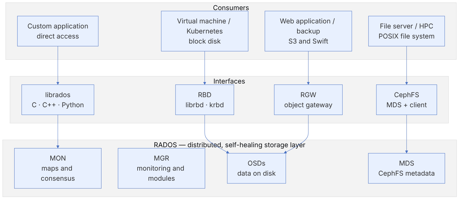
All three interfaces are built on a common layer called RADOS (Reliable Autonomic Distributed Object Store). This means replication, repair, data distribution and failure handling are implemented only once, in one place, and every interface benefits from them. Operationally, too, one cluster, one set of monitoring tools and one team are enough.
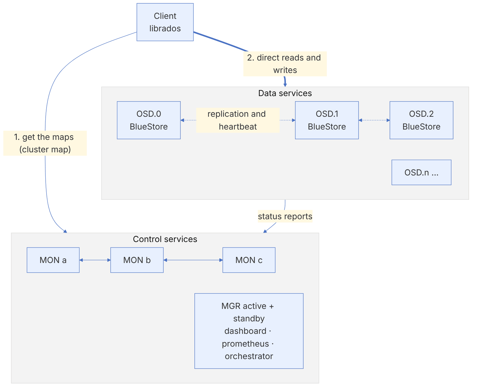
The word "Autonomic" in the name RADOS is key. In Ceph no central server decides which data must be copied where. Each OSD monitors the state of its neighbours, reports failures, and when the cluster map changes it pulls the data it needs from its peers. The MONs only hold the "map" and reach consensus on it; they are not in the data path. This design is what lets Ceph scale to thousands of OSDs.
1-2-4 Where did Ceph come from?#
Ceph grew out of Sage Weil's doctoral research at the University of California, Santa Cruz (UCSC). Its foundational papers were published in 2006: the Ceph paper at the OSDI conference and the paper on the CRUSH algorithm at the SC conference. The RADOS paper followed in 2007. The name Ceph comes from "cephalopod" (the octopus family), which is why releases are also named after animals of that family: from Argonaut and Bobtail to Reef, Squid, Tentacle and Umbrella.
| Year | Event |
|---|---|
| 2006–2007 | The Ceph, CRUSH and RADOS papers are published |
| 2010 | The CephFS client enters the Linux kernel (version 2.6.34) |
| 2012 | Inktank is founded for commercial support; the first stable release, Argonaut |
| 2014 | Red Hat acquires Inktank |
| 2017 | Luminous: BlueStore becomes stable and the default, and ceph-mgr (introduced in Kraken) becomes mandatory |
| 2018 | The Ceph Foundation is founded under the Linux Foundation |
| 2020 | Octopus: cephadm and the container-based orchestrator are introduced |
| 2023 | Red Hat's storage team (including Ceph) moves to IBM |
| 2024–2026 | Squid, Tentacle and Umbrella; FastEC, the NVMe-oF gateway, the SMB module and the Crimson preview |
Until a few years ago Jewel and Luminous were common, FileStore was the default storage engine, and installation was done with ceph-deploy. If you have read older sources, much of the difference between them and this book lies in exactly these points.
1-3 The end of the RAID era#
1-3-1 What problem did RAID solve?#
RAID was designed in the 1980s to solve a specific problem: building a disk that is bigger, faster and more reliable out of several small, cheap disks. RAID 1 with mirroring, RAID 5 with one parity and RAID 6 with two parities made it possible to survive the failure of one or two disks. At a time when disks held a few tens of gigabytes and each server had a few disks, this was an excellent solution. But over three decades disk capacity grew thousands of times while transfer speed grew only tens of times. This simple mismatch is what makes RAID inefficient at today's scale.
1-3-2 RAID rebuilds are painful#
When a disk fails in a RAID 5 or 6 array, the controller must read its contents from all remaining disks, recompute them and write them to the spare disk. The speed of this process is limited by the write speed of one disk (the spare). A 20 TB disk with a sustained rate of about 200 MB/s needs about 28 hours to fill in the best case. In practice, because the array is serving users at the same time, a rebuild usually takes several days. During all that time:
- The array runs in a degraded state, and its performance has dropped sharply.
- Fault tolerance is reduced. In RAID 5, the failure of a second disk means losing the whole array.
- All the remaining disks are under heavy read load. This is exactly the moment when disks of the same age and batch are more likely to fail.

In Ceph the data of a failed OSD is spread, in the form of hundreds of placement groups, over tens or hundreds of other OSDs. When an OSD fails, each PG is rebuilt independently on a new OSD. That means tens of disks read in parallel and tens of other disks write in parallel. This declustered recovery cuts repair time from days to minutes or a few hours, and the larger the cluster, the faster it gets.
1-3-3 Spare disks raise the cost#
To react quickly to failures, RAID needs a hot spare: a disk that has been bought, draws power, takes up space and holds no data. In a data centre with hundreds of arrays, that means hundreds of idle disks. Ceph has no concept of a spare disk. The "free capacity" of the whole cluster plays the role of the spare. You only need to plan the cluster so that after the loss of one failure domain (for example one host) it still stays below the fullness threshold. That capacity is also used for normal service in the meantime and is not wasted.
1-3-4 RAID is expensive and hardware-bound#
Hardware RAID needs a dedicated controller, a cache backed by a battery or capacitor, and often "certified" disks at a higher price. When the controller fails, often only a controller of the same model (and sometimes the same firmware version) can recognise the array again. Ceph, by contrast, sees the disks directly, without a RAID layer (JBOD or HBA mode). The intelligence is in the software, and any ordinary server with a simple HBA card is enough.
Never build Ceph OSDs on RAID 5 or RAID 6 volumes. Doing so stacks two layers of redundancy, wastes capacity, increases write latency and, most importantly, hides single-disk failure information from Ceph. If your controller has no HBA or passthrough mode, the next best option is a single-disk RAID 0 for each physical disk; in that case configure the controller's write cache carefully (and only with a healthy BBU).
1-3-5 Growing a RAID group is hard#
Adding a disk to an existing RAID group is either impossible or a long, risky operation that rewrites the whole array. In practice, organisations create a new RAID group and spread the data between groups by hand. In Ceph, adding a disk means adding an OSD. CRUSH automatically gives the new OSD a proportional share of the PGs, moving only the minimum amount of data. You can add one disk, one server or ten racks in the same way.
1-3-6 RAID's reliability model is no longer convincing#
RAID's most important weakness is statistical. Hard disks have an unrecoverable read error rate (URE) specification, usually stated as one error per bits for consumer-class disks and one error per bits for enterprise disks. bits is about 12.5 TB. Rebuilding a RAID 5 array whose healthy disks total a few tens of terabytes means reading several times that amount. The probability of hitting at least one URE during the rebuild is no longer negligible, and in RAID 5 such an error can lead to a lost block or to a complete rebuild failure.
A simple calculation of this probability is instructive. If we take the URE rate as per bit and the rebuild must read bits, the probability of finishing without an error is approximately . For reading 40 TB (about bits), is about 3.2 and the probability of finishing without an error is only about 4 percent. This figure is pessimistic, because the real rate of disks is usually better than the number on the datasheet, but it shows the direction of the trend well.
Ceph contains this problem in several ways. First, each PG is independent, so a read error affects only one object, not the whole disk. Second, with a checksum on all data (crc32c by default in BlueStore), Ceph detects silent corruption and reads the healthy copy from another peer. Third, scrub and deep scrub periodically compare all copies with each other, so hidden corruption is discovered before we need the data. Fourth, by choosing three-way replication or erasure coding with a larger m, you can pick the protection level for each pool separately.
| Aspect | RAID 6 | Ceph with 3-way replication | Ceph with EC 8+3 |
|---|---|---|---|
| Simultaneous failures tolerated | 2 disks per group | 2 failure domains (e.g. 2 hosts) | 3 failure domains |
| Capacity overhead | 2 disks out of n | 200% | about 38% |
| Rebuild bottleneck | One spare disk | The whole cluster | The whole cluster |
| Silent corruption detection | Usually limited | checksum and deep scrub | checksum and deep scrub |
| Failure domain | One server or shelf | Configurable: disk, host, rack, room | Configurable |
1-4 The Ceph architecture at a glance#
1-4-1 RADOS: the heart of the system#
Everything in Ceph is ultimately an object: an RBD disk is split into thousands of 4 MB objects, a CephFS file into data and metadata objects, and an S3 object into a head object plus its parts. RADOS is the layer that stores, replicates, distributes and repairs these objects. Every object in RADOS has a name, binary data, a number of xattrs (small key-value attributes) and an omap (a larger, sorted key-value space). The omap is where, for example, RGW keeps the list of objects in each bucket.
1-4-2 The main daemons#
| Daemon | Role | Typical count in production | Operational note |
|---|---|---|---|
| MON (ceph-mon) | Holds the cluster maps and reaches consensus with Paxos; cephx authentication | 3 or 5 (odd) | On a low-latency SSD; a majority must stay alive |
| MGR (ceph-mgr) | Statistics, modules (dashboard, prometheus, orchestrator, balancer, pg_autoscaler) | 2 (one active, one standby) | Without an active MGR, statistics and many commands do not work |
| OSD (ceph-osd) | Data storage, replication, recovery, scrub | One per disk (or several for a large NVMe) | Default memory target of 4 GB per OSD |
| MDS (ceph-mds) | CephFS file system metadata | At least one active and one standby per file system | Needed only for CephFS |
| RGW (radosgw) | HTTP gateway for S3 and Swift | Several instances behind a load balancer | Stateless; simple horizontal scaling |
Monitor (MON)#
The MONs are the cluster's "official memory". They hold a set of maps: the MON map, OSD map, PG map (in recent releases much of the PG statistics lives in the MGR), CRUSH map, MDS map (FSMap) and others. Every change to these maps is agreed among the MONs with the Paxos consensus algorithm and gets a new epoch. For the cluster to make decisions, a majority of the MONs (a quorum) must be available, which is why the number of MONs is chosen to be odd. Three MONs tolerate the failure of one, and five MONs tolerate the failure of two.
Manager (MGR)#
Since Luminous the MGR is a mandatory part of the cluster. It collects statistics about PGs, space usage and performance, and runs a set of Python modules. The web dashboard, the Prometheus exporter, the cephadm orchestrator, the balancer and the PG autoscaler are all MGR modules. At any moment only one MGR is active, and the others stay in standby.
Object Storage Daemon (OSD)#
Each OSD is usually responsible for one storage device. OSDs store data, take part in replication and recovery, exchange heartbeats with their peers and report peer failures to the MON. Since Luminous the default storage engine is BlueStore, which works directly on the raw device (chapter 12). OSDs are intelligent: they work out for themselves which PGs belong to them, and they drive peering and recovery themselves.
MDS and RGW#
The MDS is needed only for CephFS and manages the file system metadata (the directory tree, permissions, locks), while the file data itself moves directly between the client and the OSDs. RGW is an HTTP server that translates S3 and Swift requests into RADOS operations. Both are examined in detail in their own chapters (4, 5 and 6).
1-4-3 CRUSH: computation instead of lookup#
Traditional distributed storage systems rely on a central lookup table (a metadata server or name node) to find where each piece of data lives. At large scale this table is both a performance bottleneck and a point of failure. Ceph removes this table. The location of each object is computed with the deterministic CRUSH algorithm (Controlled Replication Under Scalable Hashing). Any client that has the cluster map can work out which OSDs hold the object it wants without asking any server.
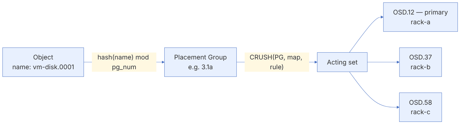
This mapping happens in two steps:
- 1. Object to PG: the object name is hashed, and its remainder modulo the number of PGs in the pool (computed stably, with a method called stable mod) determines the PG number. A PG id combines the pool number and the PG number, for example
3.1a. - 2. PG to OSDs: given the PG id, the hierarchical cluster map (racks, hosts, disks and their weights) and the pool's rule, CRUSH returns an ordered list of OSDs. The first OSD is the primary, and writes are coordinated through it.
Why is the PG layer needed? If we ran CRUSH directly on every object, each OSD would have to coordinate the state of billions of objects with its peers one by one. The PG is an aggregation layer: billions of objects are grouped into a few thousand PGs, and peering, recovery and scrub happen at the PG level. The number of PGs is a trade-off between even distribution (more PGs) and memory and CPU overhead (fewer PGs). Since Nautilus the pg_autoscaler module tunes this number automatically.
1-4-4 Pool: the unit of policy#
A pool is a logical namespace that sets the storage policy: the kind of protection (replication or erasure coding), the number of copies (size) and the minimum number of copies needed to accept I/O (min_size), the CRUSH rule (which disks and which failure domain), the number of PGs, compression and quota. Every pool also has an application tag (rbd, rgw or cephfs) that says which interface uses it.
For replicated pools, size=3 and min_size=2 are the default and the standard recommendation. Never set min_size=1 in production: the cluster may then accept writes with only one copy, and if that OSD is lost too, data the client was told was written is gone.
1-4-5 The write path of an object#
When a client writes an object to a replicated pool with size=3:
- 1. The client gets the latest OSD map from one of the MONs (if it does not already have a fresh one).
- 2. Using the hash and CRUSH, it computes the PG and the primary OSD, and sends the request directly to the primary OSD.
- 3. The primary OSD applies the write in its local transaction and, at the same time, sends it to the two secondary OSDs.
- 4. Each secondary OSD replies to the primary after it has stored the data durably.
- 5. When every copy in the acting set has made the write durable, the primary OSD sends an acknowledgement (ack) to the client.
This means Ceph has strong consistency: once a write is acknowledged, every read from any client sees the latest data. Reads are served by the primary OSD by default (although RBD and CephFS can also read from the nearest copy in certain conditions).
1-5 Planning a Ceph deployment#
1-5-1 From requirements to architecture#
Most of the costly mistakes in Ceph happen not while running it but when buying the hardware. Before anything else, these questions must be answered:
- Which interfaces? Only RBD for OpenStack or Kubernetes, only S3 for archive and backup, or a combination of all three?
- Workload pattern: small random I/O (databases, virtual machines) or large sequential I/O (video, backup, analytics data)? What is the read-to-write ratio?
- Usable capacity today and in three years, and the monthly growth rate.
- Performance targets: the required IOPS and throughput, and the acceptable 99th-percentile latency.
- Failure domain: the failure of what must be tolerated without an outage? A disk, a server, a rack, or a whole hall?
- Geographic availability: is replication to a second site needed? Synchronous or asynchronous?

1-5-2 Hardware: what does each daemon need?#
The hardware recommendations in the official Ceph documentation are a good starting point. The table below is a practical summary of them, together with common production experience:
| Component | CPU | Memory | Disk | Note |
|---|---|---|---|---|
| MON | 2 to 4 cores | At least 4 to 8 GB; more in large clusters | SSD with about 100 GB for /var/lib/ceph | Sensitive to fsync latency; avoid sharing a disk with an OSD |
| MGR | 2 to 4 cores | 4 GB or more | Negligible | Usually co-located with a MON |
| OSD on HDD | About 1 core per OSD | 4 GB (osd_memory_target) plus headroom | HDD with WAL and DB on NVMe | A typical ratio is 4 to 10 HDDs per NVMe for the DB |
| OSD on NVMe | 4 to 8 cores or more per OSD | 4 to 8 GB | Enterprise NVMe with PLP | The CPU is usually the main bottleneck |
| MDS | A fast core (single-thread speed matters) | Depends on the cache; 8 to 64 GB | Negligible | Tune mds_cache_memory_limit |
| RGW | 4 to 8 cores | 8 to 16 GB | Negligible | Several instances behind a load balancer |
Consumer SSDs without Power Loss Protection (PLP) are not suitable for Ceph. Ceph uses a flush for every durable write, and in this pattern SSDs without PLP both become very slow and may lose acknowledged data on a sudden power loss. For OSDs, DB/WAL and MONs, use only enterprise SSDs or NVMe drives with PLP.
1-5-3 Network#
Ceph is a network-centric system, and the network affects performance and stability more than any other component. There are two logical networks:
- Public network: traffic between clients and the MONs, OSDs, MDSs and RGWs. It is mandatory.
- Cluster network: replication, recovery and heartbeat traffic between OSDs. It is optional.
Recent Ceph documentation stresses that a separate cluster network is not always needed, and that in many designs a single network with enough bandwidth (for example two bonded 25 or 100 Gb links) is simpler and more reliable. If you do build a separate cluster network, it must be just as reliable as the public network. A partial failure of the cluster network can make OSDs report each other down while the MON sees them as alive, and the result is the unpleasant phenomenon known as flapping.
Keep the MTU the same along the whole path. If you enable jumbo frames (MTU 9000), they must be enabled on every NIC, bond, VLAN and switch. A single switch with a different MTU can let small packets (heartbeats) through while large packets (replication) are lost, which is one of the most confusing problems in Ceph. Test between all nodes with ping -M do -s 8972.
1-5-4 Capacity and fill ratios#
The usable capacity of a cluster must not be computed as "the sum of the disks divided by the replication factor". Three other factors must be taken into account:
- Fill ratios: by default the
nearfullwarning fires at 85%, backfill stops at 90% (backfillfull), and all writes stop at 95% (full). - Capacity needed for recovery: after the failure of the largest failure domain (for example one host), its data must fit on the rest and still stay below nearfull.
- Imbalance: even with the balancer, OSDs do not fill up exactly evenly, and the fullest OSD is what counts.
A back-of-the-envelope calculation: 6 hosts, each with 12 disks of 16 TB, three-way replication. The raw capacity is 1152 TB. If one host is lost, 960 TB remain. To stay below 80% after the failure, the raw data must not exceed 768 TB, which is about 256 TB of usable data. The same cluster with EC 4+2 (overhead 1.5) accepts about 512 TB of usable data, provided we have at least 6 hosts for a host failure domain (and preferably 7, so that recovery is possible after one host fails).
1-5-5 Failure domains and node count#
The minimum number of hosts depends on the protection policy. Three-way replication with a host failure domain needs at least three hosts, but four hosts are recommended so that, after one fails, Ceph can rebuild the third copy elsewhere. Erasure coding with a k+m profile needs at least k+m hosts, and k+m+1 is recommended for automatic repair. The more hosts there are, the smaller each one's share of the data and the smaller the impact of any single failure.
In small clusters (three or four hosts), the failure of one host means losing 25 to 33 percent of the raw capacity and a heavy recovery load on the rest. Planning the fill ratio matters twice as much in these clusters.
1-6 Building a virtual lab#
1-6-1 Lab design#
The common old approach was to use VirtualBox and Vagrant to build several virtual machines. That approach still works, but today there are lighter options too: KVM/libvirt on Linux, LXD or Incus with virtual machines, Multipass, or even a cloud server with several VMs. It does not matter which you choose; the structure we suggest is:
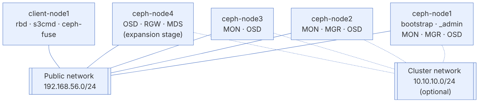
| Machine | vCPU | Memory | Disks | Role |
|---|---|---|---|---|
| ceph-node1 | 2 | 4 GB | 20 GB system + 3 disks of 20 GB | bootstrap, _admin, MON, MGR, OSD |
| ceph-node2 | 2 | 4 GB | System + 3 disks | MON, MGR, OSD |
| ceph-node3 | 2 | 4 GB | System + 3 disks | MON, OSD |
| ceph-node4 | 2 | 4 GB | System + 3 disks | Added in the "Growing the cluster" section |
| client-node1 | 1 | 2 GB | System only | RBD, S3 and CephFS client |
1-6-2 Preparing the machines#
Install a supported distribution on each node (for example Rocky Linux 9, CentOS Stream 9 or Ubuntu 24.04). According to the official documentation, the prerequisites of cephadm are: Python 3 (at least 3.9 in Umbrella), systemd, Podman or Docker, time synchronisation (chrony) and LVM2.
# On every node (example for Rocky/Alma 9)
sudo dnf install -y podman lvm2 chrony python3
sudo systemctl enable --now chronyd
# Names must be resolvable from every node
cat <<'H' | sudo tee -a /etc/hosts
192.168.56.11 ceph-node1
192.168.56.12 ceph-node2
192.168.56.13 ceph-node3
192.168.56.14 ceph-node4
192.168.56.20 client-node1
H
# Look at the empty disks (they must have no partitions or file systems)
lsblk -o NAME,SIZE,TYPE,FSTYPE,MOUNTPOINTCeph Umbrella is built on Rocky Linux 10 images, which need a CPU at the x86-64-v3 microarchitecture level. If your lab runs on virtual machines with an old or emulated CPU model (for example qemu64), the daemons will not start. In libvirt use host-passthrough, or choose the Tentacle release for the lab.
If cephadm later does not show a disk as "available", it is usually for one of these reasons: the disk has a partition or an old file-system signature, it is smaller than 5 GB, it is mounted, or it carries LVM. Use ceph orch device ls --wide to see why it was rejected (the REJECT REASONS column), and in the lab wipe it with ceph orch device zap <host> <path> --force.
1-7 Installing and configuring Ceph with cephadm#
1-7-1 Why cephadm?#
Since Octopus, cephadm has been the official tool for deploying Ceph and managing its life cycle. Three properties set it apart from the older tools:
- Containerised: each daemon runs in a Podman or Docker container with the official Ceph image. The Ceph version is independent of the operating system's package versions, and an upgrade means swapping the image.
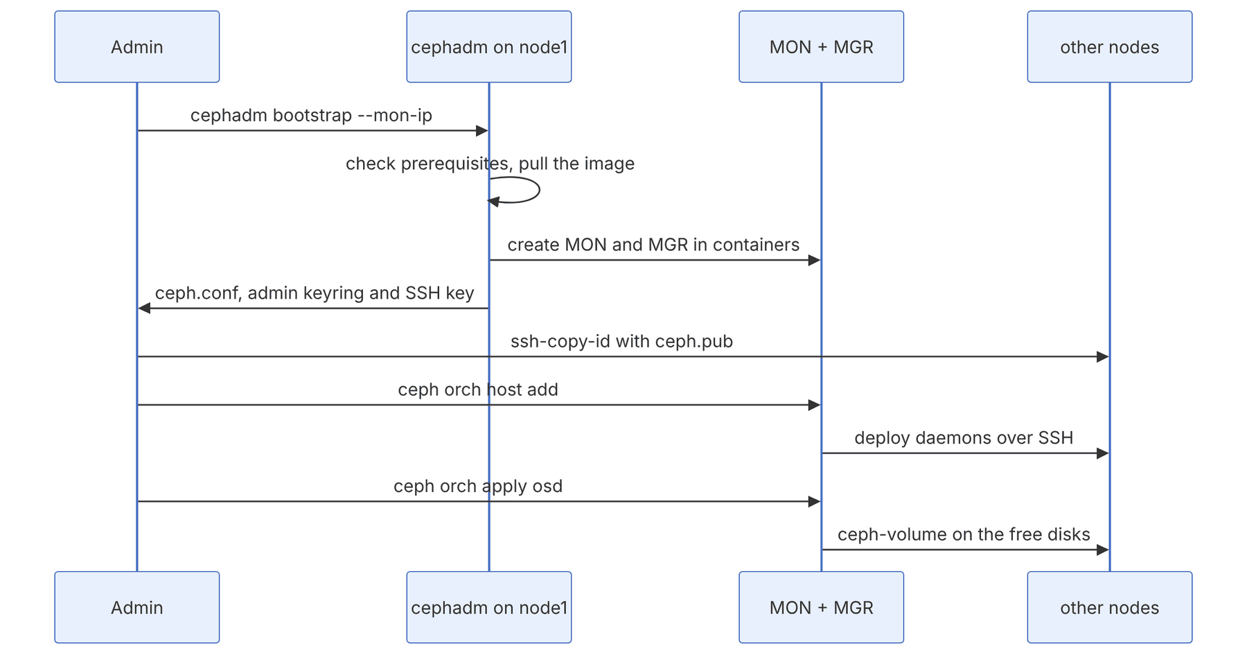
- Built-in orchestrator: cephadm runs as an MGR module and works with the hosts over SSH. You declare the "desired state" (for example "three MONs on these hosts") and the module keeps it in place, much like Kubernetes controllers.
- No external dependencies: it needs no Ansible, Salt or other configuration-management tool. Just SSH, Python and a container engine.
1-7-2 Installing cephadm and bootstrapping#
The official documentation suggests two ways of getting cephadm: the distribution package (for example apt install cephadm on Ubuntu, or the centos-release-ceph-* repository on CentOS Stream), or downloading the executable with curl. Do not mix the two methods.
# On ceph-node1 as root
CEPH_RELEASE=tentacle   # or umbrella; see the releases page for the list of active releases
curl --silent --remote-name --location \
  https://download.ceph.com/rpm-${CEPH_RELEASE}/el9/noarch/cephadm
chmod +x cephadm
./cephadm add-repo --release ${CEPH_RELEASE}
./cephadm install
which cephadm            # /usr/sbin/cephadm
Now we create the first MON and MGR. The --mon-ip address must be on the public network and reachable from every node and client:
cephadm bootstrap \
  --mon-ip 192.168.56.11 \
  --cluster-network 10.10.10.0/24 \
  --initial-dashboard-user admin \
  --allow-fqdn-hostname
When it finishes, bootstrap has done the following: created one MON and one MGR on the local host, generated a new SSH key and placed it in root's authorized_keys, written the public key to /etc/ceph/ceph.pub, put a minimal ceph.conf and the admin keyring (ceph.client.admin.keyring) in /etc/ceph, and given the bootstrap host the _admin label. The dashboard address and a temporary password are also printed in the output.
The file /etc/ceph/ceph.client.admin.keyring is the cluster's full administrative key. Anyone who has it can read or delete all data. Keep this file only on administrative hosts (those with the _admin label), never put it in a Git repository or a public backup, and create a separate user with limited access for applications (chapter 8).
1-7-3 Accessing the Ceph command line#
cephadm does not need Ceph packages installed on the host. You have two ways to run commands:
# Option 1: a shell in a container with all the tools
cephadm shell
cephadm shell -- ceph -s
# Option 2: install the command-line tools on the host
cephadm install ceph-common
ceph -v
ceph status
At this stage the output of ceph status looks something like this. The warning about the OSD count is normal, because we have not added any disks yet:
  cluster:
    id:     3f6c1d2e-....-....
    health: HEALTH_WARN
            OSD count 0 < osd_pool_default_size 3
  services:
    mon: 1 daemons, quorum ceph-node1 (age 2m)
    mgr: ceph-node1.xkqzpa(active, since 1m)
    osd: 0 osds: 0 up, 0 in
1-7-4 Adding hosts#
For the orchestrator to create daemons on other hosts, the cluster's public key must be in their authorized_keys:
ssh-copy-id -f -i /etc/ceph/ceph.pub root@ceph-node2
ssh-copy-id -f -i /etc/ceph/ceph.pub root@ceph-node3
ceph orch host add ceph-node2 192.168.56.12 --labels _admin
ceph orch host add ceph-node3 192.168.56.13
ceph orch host ls
After the hosts are added, cephadm by default spreads up to five MONs and up to two MGRs over the available hosts. In production it is better to set their placement explicitly:
ceph orch apply mon --placement="ceph-node1,ceph-node2,ceph-node3"
ceph orch apply mgr --placement="ceph-node1,ceph-node2"
ceph orch ls
ceph orch psUse labels instead of a list of host names. For example, give three hosts the mon label and run ceph orch apply mon --placement="label:mon". Later, moving a MON is just a matter of moving the label, with no need to edit the spec.
1-7-5 Adding OSDs#
The simplest way is to say that every free, suitable disk in the cluster should become an OSD:
ceph orch device ls
ceph orch apply osd --all-available-devices
# or disk by disk:
ceph orch daemon add osd ceph-node1:/dev/sdb--all-available-devices creates a persistent service: any free disk added to any host later also becomes an OSD automatically. That is convenient in a lab, but in production it may swallow a disk you attached for something else. After the initial deployment you can stop this behaviour with ceph orch apply osd --all-available-devices --unmanaged=true, or use an OSD service spec with precise filters from the start (chapter 11).
After a few minutes the cluster should reach HEALTH_OK:
ceph -s
ceph osd tree
ceph dfIf the OSDs were not created, look at ceph orch ps --daemon-type osd and ceph log last cephadm. On the target host, cephadm ls and journalctl -u ceph-<fsid>@osd.<id> give more information. Most of the time the problem is one of these: the SSH key was not added, the container image cannot be pulled (for example because of restricted internet access or no internal mirror), or the nodes' clocks are not synchronised.
In environments without direct access to quay.io, you must build an internal registry and mirror the image there, then start with cephadm --image <registry>/ceph/ceph:<tag> bootstrap .... The "Deployment in an Isolated Environment" documentation has the details.
1-7-6 Centralised configuration#
Since Mimic, Ceph configuration is kept in the MONs' configuration database instead of in ceph.conf files on each host. The ceph.conf file on the hosts holds little more than the MON addresses.
ceph config dump                          # all non-default settings
ceph config get osd osd_memory_target     # the value for one daemon type
ceph config set osd osd_max_backfills 2   # change it for all OSDs
ceph config show osd.0 | head             # the effective value on a running daemon
ceph config help osd_memory_target        # description, type and default value
During bootstrap cephadm enables automatic tuning of OSD memory (osd_memory_target_autotune), which by default divides 0.7 of the host's memory among the OSDs. On hosts that also do other work (for example in a hyperconverged setup), lower this ratio.
1-8 Growing the cluster#
1-8-1 Adding a fourth node#
One of the beauties of Ceph is that growing the cluster is a "normal operation", not a project. Prepare ceph-node4 like the others and add it:
ssh-copy-id -f -i /etc/ceph/ceph.pub root@ceph-node4
ceph orch host add ceph-node4 192.168.56.14
ceph orch host label add ceph-node4 rgw
# If the all-available-devices service is active, the disks become OSDs automatically
ceph orch device ls ceph-node4
watch -n 5 ceph -s
In the output of ceph -s you will see some PGs go into the remapped and backfilling states. CRUSH has given the new OSDs a proportional share of the PGs, and the data is being moved. The cluster stays fully available during this time.
In a production cluster holding a lot of data, adding many OSDs at once can cause a heavy wave of backfill. Since Quincy the mClock scheduler manages the recovery share automatically. If you want more control, set the norebalance flag before adding the OSDs, add them all, and then remove the flag, so that data moves only once and straight to its final destination. Tools such as upmap-remapped are also used to add weight gradually (chapter 7).
1-8-2 Adding MONs and other services#
ceph orch host label add ceph-node4 mon
# By label, but with an explicit cap of 3 instances (a YAML spec)
cat > mon.yaml <<'Y'
service_type: mon
placement:
  count: 3
  label: mon
Y
ceph orch apply -i mon.yamlDo not run an even number of MONs. Four MONs, like three, tolerate the failure of only one (a majority is 3 of 4), but they have one more voting member and one more point of failure. Either stay at 3 MONs or go straight to 5.
At this stage we can also deploy the interface services so that we can use them in later chapters:
ceph orch apply rgw demo --placement="label:rgw" --port=8080
ceph fs volume create cephfs01        # the MDSs are deployed automatically
ceph orch ls1-9 Hands-on work with the cluster#
1-9-1 Pools, objects and rados#
Let us start at the lowest layer, RADOS. We create a test pool, write a few objects to it and see where they are stored:
ceph osd pool create lab-pool
ceph osd pool application enable lab-pool rados-test
echo "salam ceph" > /tmp/hello.txt
rados -p lab-pool put hello /tmp/hello.txt
rados -p lab-pool ls
rados -p lab-pool stat hello
ceph osd map lab-pool hello
The output of ceph osd map looks something like this and shows the whole mapping path we saw in the CRUSH section: the pool and PG numbers, and the lists of up and acting OSDs, the first of which is the primary.
osdmap e87 pool 'lab-pool' (5) object 'hello' -> pg 5.4a3e9f1b (5.1b) -> up ([4,9,1], p4) acting ([4,9,1], p4)Temporarily stop one OSD of this set (ceph orch daemon stop osd.9), run ceph osd map again and look at ceph -s. The PG goes into the degraded state, but reading the object (rados -p lab-pool get hello -) still works. After about ten minutes (the default value of mon_osd_down_out_interval), the stopped OSD is marked out and recovery begins. At the end, start the OSD again: ceph orch daemon start osd.9.
1-9-2 A look at PGs and space#
ceph osd pool ls detail
ceph pg ls-by-pool lab-pool | head
ceph osd df tree
ceph df detail
ceph osd pool autoscale-status
There are two important columns in the output of ceph df: STORED (user data) and USED (the real space consumed, including replication). The MAX AVAIL column shows the writable space, taking the fullest OSD and the full ratio into account; this is the number capacity planning should be based on, not the raw sum.
1-9-3 A quick block device#
ceph osd pool create rbd
rbd pool init rbd
rbd create rbd/disk01 --size 10G
rbd info rbd/disk01
# On client-node1 (after copying ceph.conf and a suitable keyring; chapter 2)
sudo rbd map rbd/disk01
sudo mkfs.xfs /dev/rbd0 && sudo mount /dev/rbd0 /mnt
1-9-4 Cleaning up#
Deleting a pool in Ceph is deliberately hard, so that it does not happen by accident:
ceph config set mon mon_allow_pool_delete true
ceph osd pool rm lab-pool lab-pool --yes-i-really-really-mean-it
ceph config set mon mon_allow_pool_delete falseNever leave mon_allow_pool_delete permanently enabled in production. A typo in a clean-up script can delete a real pool forever. There is no "recycle bin" for pools.
1-10 From the code: from object name to bytes on disk#
1-10-1 Three layers of mapping#
Every RADOS request passes through three layers of mapping. None of them has a central "where is this object" table; everything is computed from the object name and the OSDMap. This is Ceph's most important design decision, and the rest of the chapters build on it.
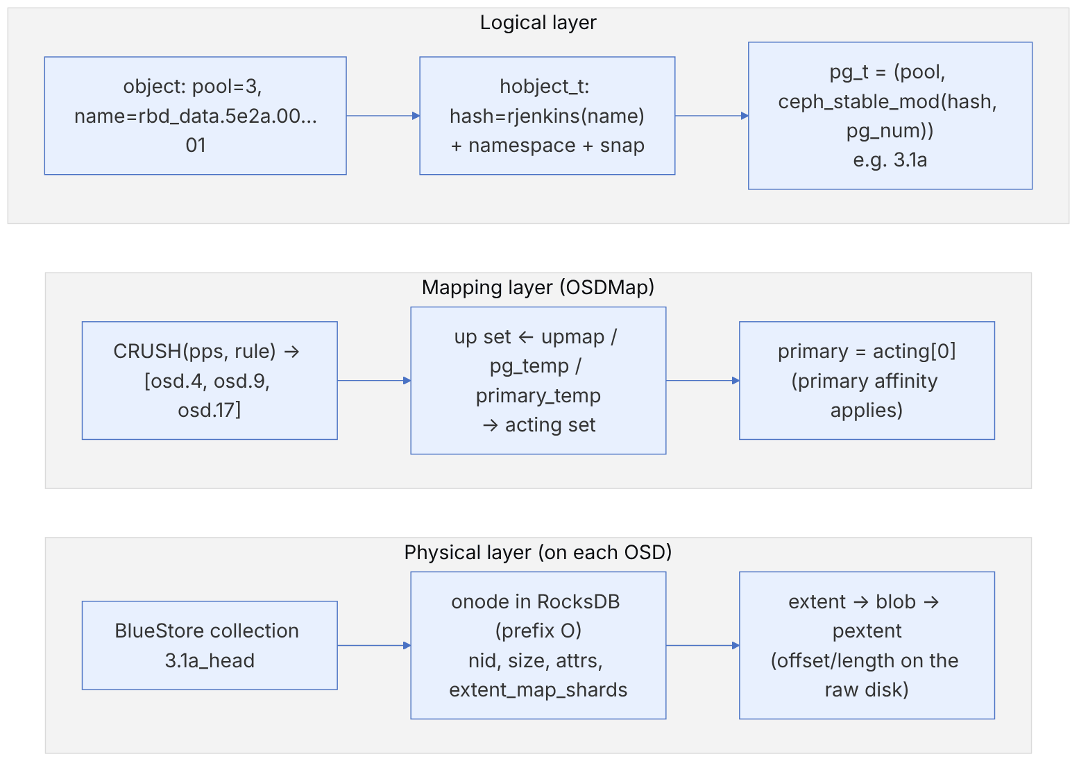
pseudocode: object → OSD (this book's summary of Objecter::_calc_target and OSDMap)
  ps      = ceph_str_hash_rjenkins(name)          # or the pool's other hash
  pg      = (pool_id, ceph_stable_mod(ps, pg_num, pg_num_mask))
  pps     = crush_hash32_2(pg.ps, pool_id)        # placement seed (different for each pool)
  raw     = crush_do_rule(rule, pps, size, weights)
  up      = apply_upmap(raw) ; drop down/out OSDs
acting = pg_temp.get(pg, up) ; primary = primary_temp.get(pg, acting[0])Run this computation yourself: ceph osd map rbd myobject follows the same path with the current OSDMap and prints the pg, up and acting. To run it offline on a copy of the map: ceph osd getmap -o om && osdmaptool om --test-map-object myobject --pool 3.
1-10-2 On-disk structures#
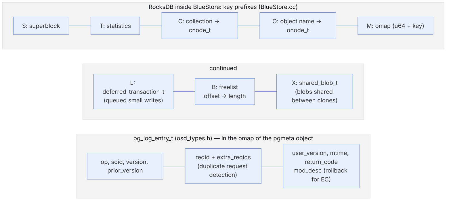
bluestore_onode_t in src/os/bluestore/bluestore_types.h has the fields nid (a unique numeric id within the OSD), size, attrs (xattrs), extent_map_shards, and the hints expected_object_size, expected_write_size and alloc_hint_flags. bluestore_blob_t is the unit of checksumming and compression, and bluestore_pextent_t is a physical range (offset and length). Blobs can be shared between clones as a bluestore_shared_blob_t.
| Constant/option | Value (main) | Why it matters |
|---|---|---|
| bluestore_min_alloc_size_hdd / _ssd | 4_K / 4_K | The smallest allocation unit; fixed when the OSD is created |
| bluestore_prefer_deferred_size_hdd / _ssd | 64_K / 0 | Smaller writes on HDD are first recorded in the WAL (deferred) |
| bluestore_max_blob_size_hdd / _ssd | 64_K / 64_K | The maximum blob size |
| bluestore_allocator | hybrid | The default allocator |
| osd_min_pg_log_entries / osd_max_pg_log_entries | 250 / 10000 | The pg log length; longer means log-based recovery instead of backfill |
| osd_target_pg_log_entries_per_osd | 300000 | The total log budget of each OSD |
The value of bluestore_min_alloc_size is recorded on the OSD at mkfs time, and changing the option on an existing OSD has no effect. Old HDD OSDs created with 64K (before Pacific) waste a lot of space for small objects such as RGW objects, and the only fix is to rebuild the OSD.
Seeing these structures in practice (stop the OSD first):
ceph osd map rbd rbd_data.5e2a.0000000000000001
ceph-objectstore-tool --data-path /var/lib/ceph/osd/ceph-4 --op list --pgid 3.1a | head
ceph-objectstore-tool --data-path ... --pgid 3.1a '<obj-json>' dump | jq '.onode'
ceph-objectstore-tool --data-path ... --op log --pgid 3.1a | jq '.pg_log_t.log[-1]'
ceph-bluestore-tool show-label --dev /dev/sdb
ceph daemon osd.4 bluestore allocator score block1-11 Planning by the numbers: PG count, the probability of data loss, and rebuild time#
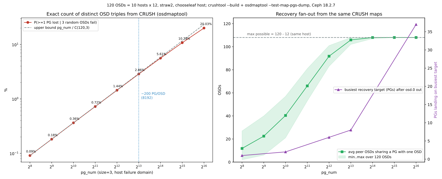
The numbers in this section come from real CRUSH mappings, not random placement. With crushtool --build --num_osds 120 … host straw2 12 root straw2 0 we built a map of 10 hosts × 12 OSDs whose default rule is chooseleaf firstn 0 type host. For each pg_num we created an osdmap with osdmaptool --createsimple 128 --pg-bits b --pgp-bits b and imported the map into it. The eight extra OSDs are not in CRUSH and receive no data. We then mapped every PG with osdmaptool --mark-up-in --test-map-pgs-dump. The tools were from Ceph 18.2.7 (Reef). The straw2 selection function (bucket_straw2_choose in src/crush/mapper.c) is the same in the main branch, so the result also holds for newer releases. The only assumption in this section is the per-disk rebuild rate, which is marked explicitly.
1-11-1 PG count and "copysets"#
Source in code: Exact computation on the CRUSH mapping with osdmaptool; default mon_target_pg_per_osd = 200 from src/common/options/mgr.yaml.in
Complexity: O(pg_num) for mapping and counting
pseudocode
for each ps in [0, pg_num): up(ps) = CRUSH(rjenkins(ps, pool), rule)   # osdmaptool --test-map-pgs-dump
S = the set of distinct (unordered) triples in up
P(loss | three random OSDs fail at the same time) = |S| / C(120, 3)          # exact, not sampled
E[fraction of PGs lost] = Σ_PG 1/C(120,3) / pg_num = 1 / C(120,3)     # independent of pg_num
Result (120 OSDs, size = 3). There are C(120, 3) = 280840 possible triples.
| pg_num | Distinct triples | Probability of losing at least one PG |
|---|---|---|
| 1024 | 1021 | 0.36% |
| 8192 (about 200 PGs per OSD) | 8037 | 2.86% |
| 65536 | 56246 | 20.0% |
At large pg_num values, the number of distinct triples falls below pg_num because of collisions. The expected fraction of data lost in such an event is exactly 1/280840 and does not depend on pg_num. Each PG is exactly one triple, and the probability that the failed triple is that one is 1/C(120,3).
The real choice is between "rarely, but a lot" and "more often, but a little". The same mappings show that with 8192 PGs the number of PGs per OSD ranges from 172 to 234. This unevenness is why the balancer and upmap exist (chapter 8).
Recovery fan-out. The same mappings show how many other OSDs each OSD shares PGs with on average. With 1024 PGs this number is about 40, and from 8192 onwards it reaches the ceiling of 108 (that is, 120 minus the 12 OSDs on the same host). So fast recovery (a short window in which three failures must coincide) matters much more than pg_num itself.
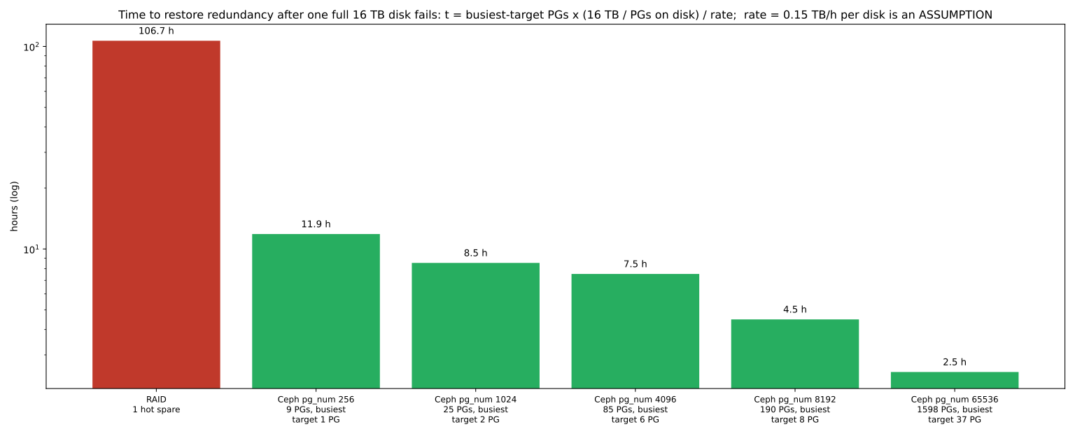
1-11-2 Declustered rebuild versus RAID#
Source in code: Mapping before and after osdmaptool --mark-out 0; real limits: osd_max_backfills, the mClock profile (chapter 21) and the network
Complexity: O(pg_num)
pseudocode
A = up before the failure ; B = up after osd.0 is marked out
moved = {pg : 0 ∈ A[pg]} ; for each pg: dst(pg) = B[pg] − A[pg]      # exactly one OSD in every case
data per PG = disk capacity / |moved|
t ≈ max_d |{pg : dst(pg) = d}| × data per PG / r                     # r = write rate of one disk (assumed)
RAID with one spare disk: t = capacity / r
Numeric example (a full 16 TB disk, assumed rate r = 0.15 TB/h). RAID takes about 107 hours. The real mapping gives these results for Ceph:
| pg_num | PGs on osd.0 | Busiest target | Time |
|---|---|---|---|
| 256 | 9 | 1 PG | 11.9 hours |
| 1024 | 25 | 2 PGs | 8.5 hours |
| 8192 | 190 | 8 PGs | 4.5 hours |
| 65536 | 1598 | 37 PGs | 2.5 hours |
In these mappings there was no collateral movement: no PG other than those of osd.0 moved. With 8192 PGs, 38 of the 190 targets (20%) were on the same host as osd.0. The reason is that "out" does not change the host's weight in CRUSH, and the retry sometimes picks the same host again.
r is an assumption, and in practice the network, osd_max_backfills or the mClock profile impose a ceiling sooner. But the structure of the result is real: the busiest target, not the average, determines the time, and a larger pg_num spreads the load more evenly. This is the main reason for dropping RAID underneath Ceph.
1-12 Supplementary and up to date#
1-12-1 From 2019 to today: what has changed?#
In 2019 the Jewel (10.2) and Luminous (12.2) releases were still common. Since then eight more major releases have come out, and several fundamental changes have happened that anyone familiar with older sources should know about:
| Topic | At the time of the book | Today |
|---|---|---|
| Deployment tool | ceph-deploy and ceph-ansible | cephadm (since Octopus) and Rook on Kubernetes; ceph-deploy is no longer maintained |
| Storage engine | FileStore by default, BlueStore new | BlueStore is the only supported option; FileStore was removed in Reef |
| Configuration | ceph.conf on every host | A centralised configuration database in the MONs (ceph config) |
| PG count | Manual calculation | pg_autoscaler by default (since Octopus) |
| I/O scheduling | WPQ with a manually tuned recovery share | mClock by default (since Quincy), with profiles |
| Network protocol | msgr v1 | msgr2 with optional encryption on port 3300 (since Nautilus) |
| Cache tiering | An active feature | Deprecated since Reef |
| Graphical management | Calamari, VSM | The Ceph Dashboard inside the MGR |
| New interfaces | — | NVMe-oF/TCP gateway for RBD, SMB module for CephFS, IAM user accounts in RGW |
| Next-generation OSD | — | Crimson and SeaStore (technical preview) |
1-12-2 Active releases at the time of writing#
According to the official releases page (visited November 2026), three stable releases are actively maintained: Umbrella (21.2, first released on 28 October 2026), Tentacle (20.2, first released on 18 November 2025; the latest version at the time of writing is 20.2.5) and Squid (19.2, with an estimated end of life on 2 December 2026). Reef is now archived. Ceph publishes one major release a year, and X.2.Z versions are the stable releases meant for production (X.1.Z are release candidates and X.0.Z are development points).
A common production policy is to stay on the previous major release until several point releases of the new one have been published. For example, at the time of writing, Tentacle with five point releases is a more conservative choice than Umbrella, which was released only a few weeks ago. Read the release notes in full before upgrading, especially the sections that change defaults.
Umbrella changes several defaults that can alter the cluster's behaviour after an upgrade: the default mon_target_pg_per_osd has gone from 100 to 200 and mon_max_pg_per_osd from 250 to 500, so existing pools may autoscale to more PGs after the upgrade. For clusters whose OSD memory target is below 4 GB, or whose SSDs are split into more than two OSDs, the release notes suggest pinning the old values explicitly before upgrading.
1-12-3 Rook: Ceph on Kubernetes#
If your infrastructure is Kubernetes, Rook is the official CNCF operator (a graduated project) for running Ceph on Kubernetes. Rook runs the same Ceph daemons as Pods and exposes resources such as CephCluster, CephBlockPool, CephObjectStore and CephFilesystem as CRDs. At the time of writing, the latest Rook release is 1.21.2. cephadm and Rook both build on the shared concepts of the Ceph orchestrator, but choose only one of them for a given cluster.
1-12-4 When is Ceph not the right choice?#
Ceph is a powerful tool, but it is not right for every problem:
- Very small clusters: below three or four hosts, Ceph's operational overhead and wasted capacity are usually not justified. A simple NAS or ZFS is better.
- Very low latency for a single application: every write in Ceph needs at least one network round trip to the primary OSD and one to the secondaries. For a database that needs latency below 100 microseconds, local NVMe with application-level replication is a better option.
- A team without operational experience: Ceph behaves well under failures, provided someone knows what to do in unusual situations. Investing in training and monitoring is part of Ceph's real cost.
1-13 Summary and review#
1-13-1 Chapter summary#
- Software-defined storage separates intelligence from hardware and makes horizontal scaling, vendor independence and unified interfaces possible.
- At the scale of multi-terabyte disks, RAID hits a dead end with many-to-one rebuilds, spare disks and URE risk; Ceph solves these problems with many-to-many recovery, checksums and scrubbing.
- All Ceph interfaces (RBD, RGW, CephFS) are built on RADOS. The MONs hold the map, the MGR holds statistics and modules, and the OSDs hold the data.
- CRUSH computes where data lives; there is no central table. An object maps to a PG, and a PG maps to a set of OSDs in different failure domains.
- Correct planning (workload type, failure domain, network, fill ratio, SSDs with PLP) is the most important factor in Ceph's success.
- cephadm is today's official deployment tool: bootstrap, add hosts, and declare the desired state with
ceph orch apply.
1-13-2 Common mistakes#
- Building OSDs on RAID 5/6, or on virtual disks that sit on one shared physical disk.
- Using consumer SSDs without PLP for DB/WAL or MONs.
- Setting
min_size=1to "stay up" during a failure. - Inconsistent MTU along the network path.
- An even number of MONs, or putting all MONs in one rack.
- Planning capacity from the raw capacity without accounting for nearfull and the loss of the largest domain.
- Leaving the
all-available-devicesservice running in production.
1-13-3 Self-assessment checklist#
- I can explain Ceph's three interfaces and their common layer.
- I know what the MON, MGR, OSD, MDS and RGW each do, and how many of each are needed.
- I can show the object → PG → OSD path with
ceph osd map. - I can build a three-node cluster with cephadm and add a fourth node.
- I can estimate the usable capacity of a design, taking replication, failures and nearfull into account.
1-13-4 Hands-on exercise#
- 1. Build this chapter's four-node lab and bootstrap the cluster with three nodes. Save the output of
ceph -sandceph orch ps. - 2. Create a replicated pool, write 100 small objects to it with a bash loop (
for i in $(seq 1 100); do rados -p lab-pool put obj$i /etc/hosts; done) and look at their distribution across PGs withceph pg ls-by-pool. - 3. Add the fourth node and follow the backfill with
ceph -s. What percentage of the PGs moved? Why did not all of them move? - 4. Stop one OSD and measure the time until it is marked
outand recovery finishes. Then lowermon_osd_down_out_intervalto 60 seconds in the lab and repeat the test. - 5. Compute the usable capacity of your own design for two scenarios, three-way replication and EC 4+2, with the condition of staying below 80% after the loss of one host.
1-13-5 Review questions#
- 1. What are the three fundamental limitations of traditional storage arrays that software-defined storage removes?
- 2. Why does RAID rebuild time get worse as disks get bigger, while Ceph recovery time gets better as the cluster gets bigger?
- 3. Compare the roles of the MON and the OSD in the write path of an object. Does data pass through the MON?
- 4. What problem does the PG layer solve, and what would happen if it did not exist?
- 5. Why is the number of MONs chosen to be odd? How many failures do four MONs tolerate?
- 6. What is the difference between
sizeandmin_size, and why ismin_size=1dangerous? - 7. When is a separate cluster network useful, and what risk does it carry?
- 8. Why is an SSD without PLP unsuitable for Ceph?
- 9. Which files does cephadm create in
/etc/cephduring bootstrap, and which one is the most sensitive? - 10. Which two Umbrella default changes can alter the cluster's behaviour after an upgrade?
Answers to these questions are in Appendix E: Answers to Review Questions. Answers to this chapter's questions →
1-13-6 Sources for this chapter#
- Ceph documentation — Architecture
https://docs.ceph.com/en/latest/architecture/ - Ceph documentation — Hardware recommendations
https://docs.ceph.com/en/latest/start/hardware-recommendations/ - cephadm documentation — Deploying a new cluster
https://docs.ceph.com/en/latest/cephadm/install/ - cephadm documentation — Host management
https://docs.ceph.com/en/latest/cephadm/host-management/ - cephadm documentation — Service specifications and placement
https://docs.ceph.com/en/latest/cephadm/services/ - Ceph documentation — Network configuration
https://docs.ceph.com/en/latest/rados/configuration/network-config-ref/ - Ceph documentation — Releases and the release cycle
https://docs.ceph.com/en/latest/releases/ - Umbrella release notes
https://docs.ceph.com/en/latest/releases/umbrella/ - Tentacle release notes
https://docs.ceph.com/en/latest/releases/tentacle/ - Weil et al., "Ceph: A Scalable, High-Performance Distributed File System", OSDI 2006
https://www.usenix.org/legacy/event/osdi06/tech/weil.html - Weil et al., "CRUSH: Controlled, Scalable, Decentralized Placement of Replicated Data", SC 2006
https://ceph.io/assets/pdfs/weil-crush-sc06.pdf - Weil et al., "RADOS: A Scalable, Reliable Storage Service for Petabyte-scale Storage Clusters", PDSW 2007
https://ceph.io/assets/pdfs/weil-rados-pdsw07.pdf - Rook documentation
https://rook.io/docs/rook/latest-release/